


Here are some physics simulations and artwork along with some Mathematica code. See also my Fluid Motion page.
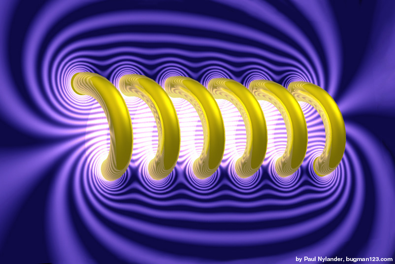
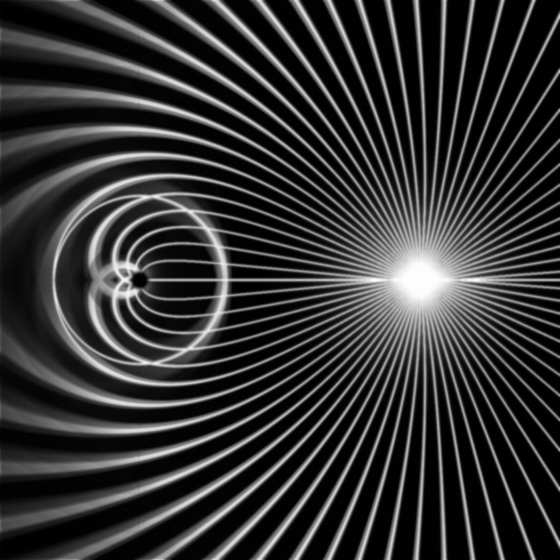
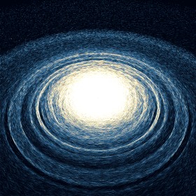
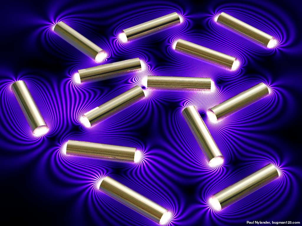
Magnetic Field of a Solenoid - new version: POV-Ray 3.6.1, 5/17/06
old version: calculated in Mathematica 4.2, rendered in TrueSpace 4.3, 1/19/03

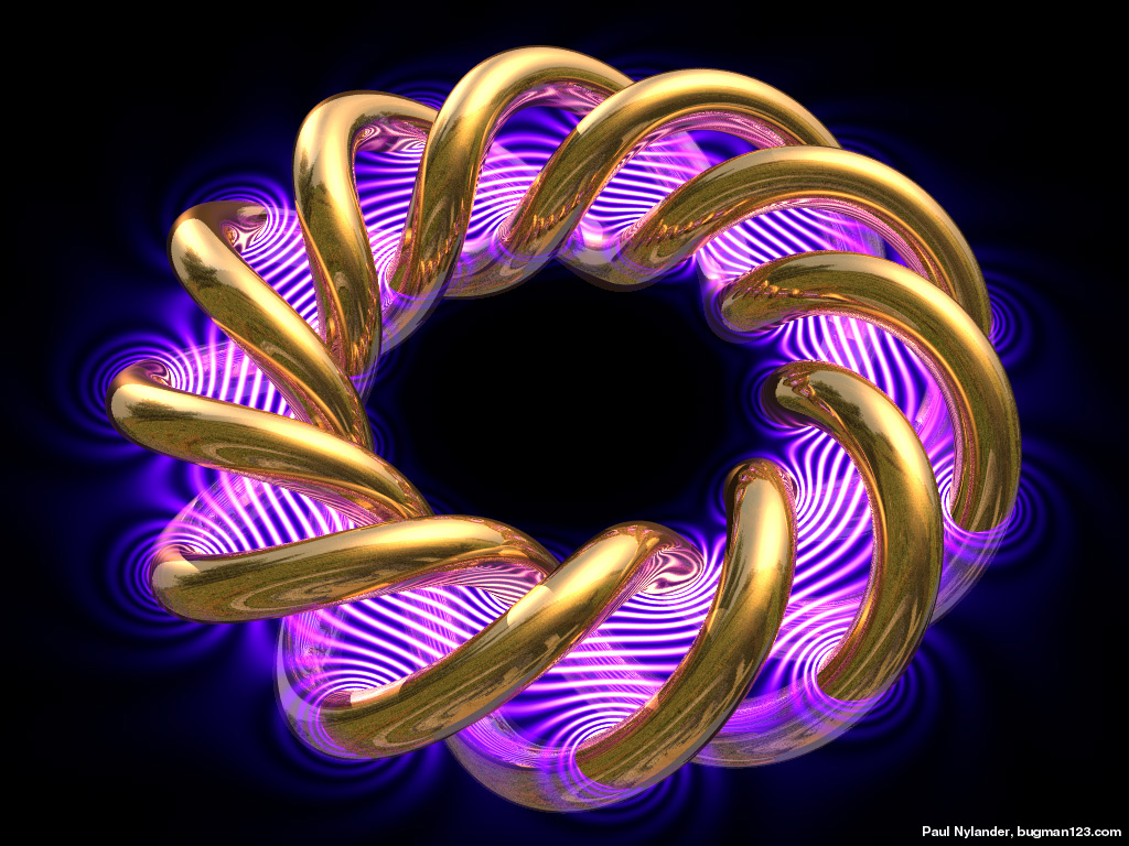


 This magnetic field was approximated by a superposition of 2D point sources using the Biot-Savart Law. Click here to download the POV-Ray code for this image. See also my magnetic field representations for a motor, Tesla coil, and horseshoe magnets. Here is some Mathematica code: (* runtime: 12 seconds *) plist = Table[{(4 i - 26)/6, -(-1)^i}, {i, 1, 12}]; r[{xi_, yi_}] := Sqrt[(x - xi)^2 + (y - yi)^2]; DensityPlot[2Sqrt[((Plus @@ Map[#[[2]](x - #[[1]])/r[#]^2 &, plist])^2 + (Plus @@ Map[-#[[2]](y - #[[2]])/r[#]^2 &, plist])^2)] + Cos[18.8Plus @@ Map[#[[2]]/r[#] &, plist]] + 1, {x, -6, 6}, {y, -3, 3}, Mesh -> False, Frame -> False, PlotRange -> {0, 10}, PlotPoints -> {275, 138}, AspectRatio -> 1/2] This image was featured on the September 2009 cover of Physics Today magazine. You can also see an older version of this picture on Jeff Bryant’s Mathematica visualization site. Links Large Helical Deivce - beautiful fusion stellarator in Japan |
2D Wave-Particle Simulations - Mathematica 4.2, 1/15/05; C++ version: 5/16/07
 The left animation shows the quantum mechanical probabilty distribution of an electron as it passes through two narrow slits. The electron itself is much smaller than its probability distribution cloud, which is dispersed over a large area, creating an interference pattern. However, when the electron is observed, then its probability distribution cloud will become small again. The following Mathematica code uses the Crank-Nicolson method with time-splitting to solve the Schrödinger wave equation. I learned this technique from Terry Robb's Mathematica notebook: (* runtime: 10 seconds, V is the potential energy *) << LinearAlgebra`Tridiagonal`; n = 55; dx = 1.0/(n - 1); hbar = m = 1; dt = 2m dx^2/hbar; a = I hbar/dt; b = hbar^2/(4 m dx^2); blist = Table[b, {n - 1}]; psi = Table[Module[{p = {x - 0.25, y - 0.5}}, Exp[I {100, 0}.p - p.p/(2 0.14^2)]], {y, 0, 1, dx}, {x, 0, 1, dx}]; V = Table[If[0.48 < x < 0.52 && ! (0.4 < y < 0.475 || 0.525 < y < 0.6), 10000, 0], {y, 0, 1, dx}, {x, 0, 1, dx}]; Do[psi = Table[TridiagonalSolve[blist, 2a - 2b - V[[All, j]]/2, blist, (2a + 2b + V[[All, j]]/2)psi[[All, j]] - b Table[psi[[i, Min[n, j + 1]]] + psi[[i, Max[1, j - 1]]], {i, 1, n}]], {j, 1, n}]; psi = Table[TridiagonalSolve[blist, 2a - 2b - V[[i,All]]/2, blist, (2a + 2b + V[[i, All]]/2)psi[[All, i]] - b Table[psi[[j, Min[n, i + 1]]] + psi[[j, Max[1, i - 1]]], {j, 1, n}]], {i, 1, n}]; Show[Graphics[RasterArray[Map[(x = Min[Abs[#]^2, 1];Hue[Arg[#]/(2Pi), Min[1, 2(1 - x)], Min[1, 2x]]) &, psi + V, {2}]], AspectRatio -> 1]], {40}]; |
 The color in these pictures represents the complex phase. Here is some Mathematica code in case you’re wondering how TridiagonalSolve works:
TridiagonalSolve[a_, b_, c_, r_] := Module[{n = Length[r], p, q}, p = q =Table[0, {n}]; {p[[1]], q[[1]]} = {c[[1]], r[[1]]}/b[[1]]; Do[{p[[i]], q[[i]]} = {If[i < n, c[[i]], 0], r[[i]] - a[[i - 1]]q[[i - 1]]}/(b[[i]] - a[[i - 1]]p[[i - 1]]), {i, 2, n}]; Do[q[[i]] -= p[[i]]q[[i + 1]], {i, n - 1, 1, -1}]; q]; Links Advanced Visual Quantum Mechanics - nice animations Shroedinger simulator - C++ program by Maciej Matyka high energy quantum eigenfunctions in hyperbolic space - unexplained patterns by Dennis Hejhal |
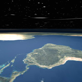
Special Relativity - C++, POV-Ray 3.6.1, Mathematica 4.2, 8/25/09
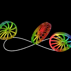


 What would everyday life look like if the speed of light was very slow? According to Einstein’s theory of Special Relativity, moving objects would be Lorentz contracted. Moving objects would also appear distorted if light arriving from one part of the object was emitted at a different instant in time than light arriving from another part. And the Doppler effect would cause approaching objects to look more blue and receding objects to look more red. These simulations were inspired from Ute Kraus' and Corvin Zahn's Rolling Wheels animations. (Note: I am not yet certain if the distortion in my simulations is exactly correct here.)
Links Space Time Travel - animations by Ute Kraus and Corvin Zahn, be sure to see the Rolling Wheels and Through the city animations Relativistic Flight through a Lattice - simple Java applet with source code, by Ute Kraus and Corvin Zahn Real-time Relativistic Rendering - by Hansong Zhang Lorentz-Fitzgerald Contraction / Penrose-Terrell Rotation |
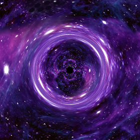
Simulation of Earth as a Black Hole - C++, 8/27/09
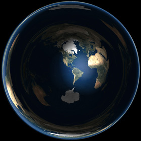


 This ray traced image was inspired from Werner Benger's simulation of Earth as a black hole. The reason for using Earth in this example is to provide a familiar reference point to help you perceive the distortion. The first animation shows rotation, the second animation shows the mass steadily increasing while everything else is kept stationary (notice the Einstein ring in the stars), and the third animation shows what a viewer would see while in orbit at the photon sphere. Technically, the Earth would become invisible once the Schwarzschild radius exceeded the Earth's actual radius, but I am ignoring that here.
Links Black Hole Raytracing - by Werner Benger Virtual Trips to Black Holes - simulations by Robert Nemiroff Black Hole Simulation - by Phil Armitage Black Hole Flight Simulator - screenshots and Java applet, by Andrew Hamilton Reissner-Nordstroem - solution for electrically charged black hole, spherically symmetric, has two nested event horizons and gravitationally repulsive timelike singularity at center that cannot be reached (similar to rotating black hole) |
Pool Simulations - Mathematica version: 7/9/05, C# version: 10/27/10, rendered in POV-Ray 3.6.1
 Here’s a fun one. The instant when the cue ball breaks a tightly-packed triangle, the inner balls must rapidly bounce around until they spread out. These simulations include rotational effects, however the following simple Mathematica code does not: (* runtime: 2 seconds *) Normalize[p_] := p/Sqrt[p.p]; Assoc[x_, data_] := Flatten[Select[data, #[[1]] == x &], 1]; r = 1.125; xmax = 50; ymax = 25; n = 16; balls = Prepend[Flatten[Table[{{xmax/2 + 1.05Sqrt[3]x, 1.05y}, {0, 0}}, {x, 4r, 0, -r}, {y, -x, x, 2r}], 1], {{-xmax/2 - 1.1r, 0}, {100, 0}}]; Step[dt0_] := Module[{dt = dt0, collisions = {}}, Do[{pa1, va} = balls[[i]]; pa2 = va dt0 + pa1; Do[If[j != i, {pb1, vb} = balls[[j]]; pb2 = vb dt0 + pb1; p1 = pa1 - pb1; p2 = pa2 - pb2; p = p1 - p2; a = p.p; b = -2p1.p; c = p1.p1 - (2r)^2; d = b^2 - 4a c; If[d >= 0, t = If[a == 0, If[b == 0, 1, -c/b], Min[(-b + {1, -1}Sqrt[d])/(2a)]]; If[0 <= t dt0 <= dt, pa = (1 - t)pa1 + t pa2; pb = (1 - t)pb1 + t pb2; normal = Normalize[pa - pb]; va -= (va - vb).normal normal; If[t dt0 < dt, dt =t dt0; collisions = {{i, va}}, collisions = Append[collisions, {i, va}]]]]], {j, 1, n}], {i, 1, n}]; balls = Table[{pa1, va1} = balls[[i]]; temp = Assoc[i, collisions]; {va1 dt + pa1, If[temp != {}, temp[[2]], va1]}, {i, 1, n}]; If[dt < dt0, Step[dt0 - dt]]]; Do[Show[Graphics[Map[Disk[#[[1]],r] &, balls], PlotRange -> {{-xmax, xmax}, {-ymax, ymax}}, AspectRatio -> 0.5]]; Step[0.1], {50}]; Links Deep Green and ARPool - pool playing robot and augmented reality pool system, by RCVLab at Queen's University Pool Project - useful formulas by Brian Townsend, see also his page on The Math and Physics of Billiards Amazing Snooker Plant - YouTube video Pool Simulations |


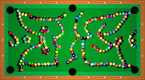
Pool Fractal: "1 Million Games of Pool" - calculated in C#, rendered in POV-Ray 3.6.1, 10/27/10
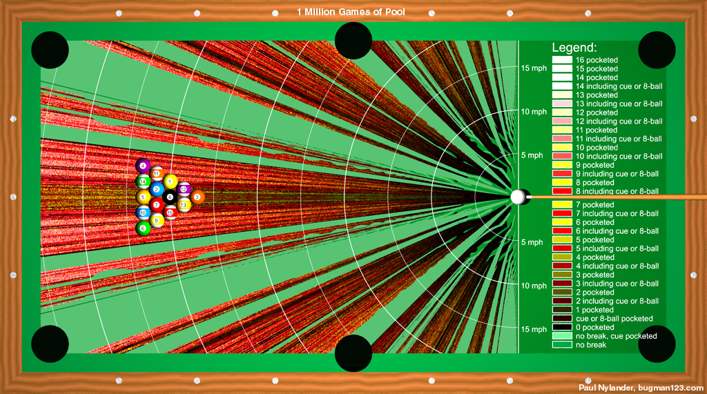
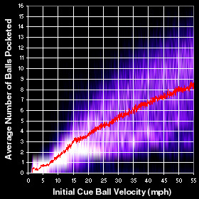 I've heard people tell me that there are professional pool players who can pocket a full triangle of 15 tightly packed billiard balls on a single break. But based on what I read in this article, it sounds unlikely that anyone can pocket more than 7 balls on the break. However, if the cue ball was struck with superhuman speed, then perhaps it might be possible to pocket all the balls, because the balls would move greater distances, thereby covering more territory (I think this would be an interesting experiment for Myth Busters to test). In order to test this theory, I simulated many different breaks, by launching the cue ball at various speeds and angles. The slowest scenario I found that could pocket all the balls had a cue ball initial speed of 34 mph (real life players can strike the cue ball up to about 27 mph). The fractal image on the left summarizes the results. You may notice from this image that your best bet is to aim off-center if you want to pocket as many balls as possible.
|
Magnetic Pool - calculated in C#, rendered in POV-Ray 3.6.1, 10/27/10
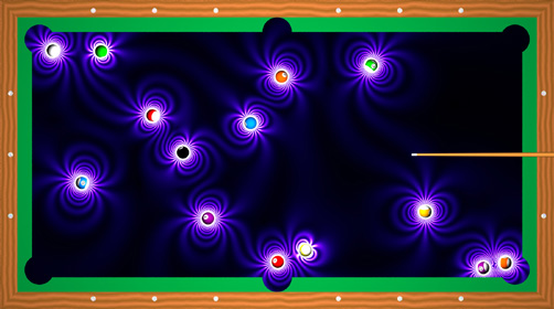 Suppose you had a special pool table that could visualize the magnetic field of magnetized billiard balls on the surface of the table. But that's cheating you say? True, but it would also make an interesting way to study the physics of magnetism. Perhaps something like this could be created for a children's science museum. The magnetic field in these simulations was calculated using the simple formula for the magnetic field of uniformly magnetized spheres and the forces and torques were calculated using the formulas for induced force and torque on small magnets.
Links Magnets in Motion - impressive magnetics simulations paper and video Network - magnetic field visualizations of magnetized spheres, by Daniel Walsh amazing and educational magnetic spheres - you can buy 216 Nanodots for $30, 224 NeoCube spheres for $25, or 216 Buckyballs for $30 |
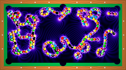
 If you increase the magnetic field strength and the number of billiard balls, interesting structures can emerge, similar to the way molecules are formed.
|
|
3D Collisions - calculated in Mathematica 4.2, rendered in POV-Ray 3.6.1, 7/9/05
 Here is a box of frictionless bouncy balls with gravity. The balls don’t rotate and never stop bouncing because there is no friction. This simulation uses the same basic Mathematica code as the pool table simulation shown above.
(* runtime: 52 seconds *) << Graphics`Shapes`; g = {0, 0, -9.80665}; xmax = 1; Normalize[p_] := p/Sqrt[p.p]; Distance[p1_, p2_] := Sqrt[(p2 - p1).(p2 - p1)]; Move[{p_, v_}, t_] := {g t^2/2 + v t + p,g t + v}; Interpolate[t_, x1_, x2_] := (1 - t)x1 + t x2; Step[dt_] := Module[{particles2 = Table[{pa1, va1} = particles[[i]]; {pa2, va2} = Move[{pa1, va1}, dt]; result = {pa2, va2}; tmin = Infinity; Do[If[j != i, {pb1, vb1} = particles[[j]]; {pb2, vb2} = Move[{pb1, vb1}, dt]; p1 = pa1 - pb1; p2 = pa2 - pb2; p = p1 - p2; a = p.p; b = -2p1.p;c = p1.p1 - (2r)^2; d = b^2 - 4a c; If[d >= 0, If[a == 0, t = If[b == 0, 1, -c/b], t = (-b + {1, -1}Sqrt[d])/(2a); t = If[0 <= Min[t] <= 1, Min[t], t[[If[0 <= t[[1]] <= 1, 1, 2]]]]]; If[0 <= t <= 1 &&t < tmin, tmin = t; pa = Interpolate[t, pa1, pa2]; pb =Interpolate[t, pb1, pb2]; va = Interpolate[t, va1, va2]; vb = Interpolate[t, vb1, vb2]; normal = Normalize[pa - pb]; va -= (va - vb).normal normal;result = Move[{pa, va}, (1 - t)dt]]]], {j, 1, n}];Do[If[va1[[dim]] != 0, Scan[Module[{t = (#(xmax - r) - pa1[[dim]])/(va1[[dim]]dt)}, If[0 <= t <= 1 && t < tmin, tmin = t;pa = Interpolate[t, pa1, pa2]; va = Interpolate[t, va1, va2]; va[[dim]] = -va[[dim]];result = Move[{pa, va}, (1 - t)dt]]] &, {-1, 1}]], {dim, 1, 3}]; result, {i, 1, n}]},collision = False; Do[pa2 = particles2[[i, 1]]; If[Min[pa2] < -(xmax - r) || Max[pa2] > xmax -r, collision = True]; Do[If[Distance[particles2[[j, 1]], pa2] < 2r, collision = True], {j, i + 1, n}], {i, 1, n}]; If[collision, Do[Step[dt/2], {2}], particles = particles2]]; r = 0.25; n = 20; particles = {}; SeedRandom[0]; Do[start = True; While[start || Or @@ Map[Distance[p, #[[1]]] < 2r &, particles], start = False; p = (xmax - r)Table[2 Random[] - 1, {3}]];particles = Append[particles, {p, {0, 0, 0}}], {n}]; Do[Step[0.05]; Show[Graphics3D[{EdgeForm[], Map[TranslateShape[Sphere[r, 10, 6], #[[1]]] &, particles]}, PlotRange -> xmax{{-1, 1}, {-1, 1}, {-1, 1}}]], {50}]; Collision Links Crayon Physics Deluxe - real-time 2D sketched simulations, by Petri Purho, uses the Box2D open source physics engine by Erin Catto Crayon Physics - real-time 2D sketched simulations, by Phun - real-time 2D sketched simulations, by Emil Ernerfeldt Box2DJS - JavaScript program Collision Detection - similar program by Jason Stewart Rigid Body Animations - by Eran Guendelman, Ron Fedkiw, and Robert Bridson Rigid Body Dynamics - Pixar notes by David Baraff JuggleMaster - fun Java applet, originally by Ken Matsuoka |
Raindrop Light Refraction & Dispersion - Mathematica 4.2, 1/21/05; C++ version: 7/26/05
 When light enters near the side of a raindrop, much of the light is internally reflected. This is how rainbows are formed. Click here to see a YouTube video using this animation by Dianna (Physics Girl). Click here to see some POV-Ray code for a similar-looking image using photon mapping. Here is some Mathematica code:
(* runtime: 12 seconds *) Spectrum = {{380, {0, 0, 0}}, {420, {1/3, 0, 1}}, {440, {0, 0, 1}}, {490, {0, 1, 1}}, {510, {0, 1,0}}, {580, {1, 1, 0}}, {645, {1, 0, 0}}, {700, {1, 0, 0}}, {780, {0, 0, 0}}}; Snell[theta_, n1_, n2_] := ArcSin[Min[1, Max[-1, Sin[theta]n1/n2]]]; FresnelR[t1_, t2_, n1_, n2_] := (((n1 Cos[t2] - n2 Cos[t1])/(n1 Cos[t2] + n2 Cos[t1]))^2 + ((n1 Cos[t1] - n2 Cos[t2])/(n1 Cos[t1] + n2 Cos[t2]))^2)/2; Angle[{x1_, y1_}, {x2_, y2_}] := ArcTan[x2 - x1, y2 - y1]; IntersCircle[{x_, y_}, theta_, {x0_,y0_}, r_] := Module[{t1 = Tan[theta], t2, a, b, x2}, t2 = ((x -x0) t1 - (y - y0))/r; a = t1^2 + 1; b = -2t1 t2; x2 = x0 + r(-b + If[Cos[theta] > 0, 1, -1]Sqrt[b^2 - 4a (t2^2 - 1)])/(2a); {x2, y + (x2 - x)t1}]; AddLine[{x1_, y1_}, {x2_, y2_}, color_] := Do[image[[Round[m(s y1 + (1 - s) y2)], Round[m(s x1 + (1 - s)x2)]]] += color, {s, 0,1, 1/(m Sqrt[(x2 - x1)^2 + (y2 - y1)^2])}]; m = 275; image =Table[{0, 0, 0}, {m}, {m}]; x0 = y0 = 0.5; p0 = {x0, y0}; r = 0.25; y = y0 + r - 0.0001; Do[n = 1.31Exp[12.4/lambda];color = Table[Interpolation[Map[{#[[1]], #[[2, i]]} &, Spectrum], InterpolationOrder -> 1][lambda], {i, 1, 3}]; p1 = {x0 - Sqrt[r^2 - (y - y0)^2], y}; t = Angle[p0, p1]; t1 = t + Snell[Pi - t, 1, n] - Pi; While[Max[color] > 0.01, p2 = IntersCircle[p1, t1, p0, r]; AddLine[p1,p2, color]; t = Angle[p0, p2]; t2 = 2t - t1 - Pi; t3 = t - Snell[t - t1, n, 1]; R1 = FresnelR[t - t1, t - t3, n, 1]; AddLine[p2, IntersCircle[p2, t3, p0, 0.49], (1 - R1) color]; p1 = p2; t1 = t2; color *= R1], {lambda, 380, 780, 25}]; Show[Graphics[RasterArray[Map[RGBColor @@ Map[Min[1, #] &, #] &, image, {2}]], Epilog -> {{RGBColor[1, 1, 1], Circle[m p0, m r]}}, AspectRatio -> 1]] Links: Prism HD - fun and beautiful iPhone app, very similar to this, by Orion Elenzil Crazy Dispersion - reverse dispersion, by Thomas Ludwig Fire Rainbow - rare & beautiful atmospheric phenomenon |
Diamond Light Refraction & Dispersion - Mathematica 4.2, 1/29/05
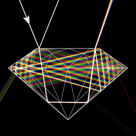
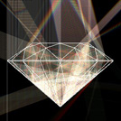 Diamonds have a high index of refraction (n = 2.4195) and coefficient of dispersion (COD = 0.044). When light reaches a boundary, it can refract or reflect, in proportion to the Fresnel Reflection Coefficient. The angle of the refracted light is given by Snell’s Law: n1sin(θ1) = n2sin(θ2). See also Sellmeier equation.
Links Click here to see my rock and gemstone collection. Ray Traced Diamond - POV-Ray code by PM 2Ring, based on Marcel Tolkowsky’s “ideal” diamond Raytracing Diamonds - paper by Sabine Fischer Prism Refraction - Java applet Metamaterials - materials with negative index of refraction may be used to create Cloaking devices, cloaking carpet |
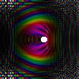
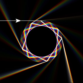
Photon Sphere - Mathematica 4.2, 8/21/09
 At just the right distance from the center of a black hole, light can orbit the black hole in a circular orbit called a photon sphere. The radius of the photon sphere is 1.5 times larger than the Schwarzschild radius, inside which nothing can escape. This image shows the paths of light rays from a point source near a black hole. The above differential equation for the light ray's path was derived from the Schwarzschild metric. Here is some Mathematica code to solve this equation using the 4th order Runge-Kutta method: (* runtime: 0.4 second *) m = 0.098691; dphi = Pi/180.0; f[{u_, du_}] := {du, 3m u^2 - u}; Runge[x_] := Module[{k1, k2, k3, k4}, k1 = dphi f[x]; k2 =dphi f[x + k1/2]; k3 = dphi f[x + k2/2]; k4 = dphi f[x + k3]; (k1 + 2k2 + 2k3 + k4)/6]; paths = Table[r = 1; phi = 0; u = 1/r; du = -Cot[theta]/r; path = {}; While[0.01 < r < 2, {u, du} += Runge[{u, du}]; r = 1/u; path = Append[path, r{Cos[phi], Sin[phi]}]; phi += dphi]; path, {theta, 0.0, Pi, Pi/36}]; Show[Graphics[Map[Line, paths], AspectRatio -> 1, PlotRange -> {{-0.5, 1.5}, {-1, 1}}]] |
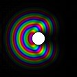
Einstein Ring - Mathematica 4.2, 2/5/05
 According to Einstein’s General Theory of Relativity, the intense gravity of a black hole can bend light into a circle called an Einstein Ring. The following Mathematica code is only an approximation:
(* runtime: 30 seconds *) Clear[stars]; SeedRandom[535]; stars[{x_, y_}] = Sum[Exp[-500((x - Random[])^2 + (y - Random[])^2)/Random[]^2], {10}]; DensityPlot[Module[{r = x^2 + y^2}, If[r < 0.1^2, 0, stars[Mod[0.5((1 - 0.25/r) {x, y} + 1), 1]]]], {x, -1, 1}, {y, -1, 1}, PlotPoints ->275, PlotRange -> {0, 1}, Mesh -> False, Frame -> False] Links Einstein Ring Animation, Stereoscopic Visualization of Curved Space - by Werner Benger Relativistic Black Hole Plug-in for Maya - by Marcel Ritter, see also his paper "Monster of the Milky Way" - Nova video about black holes Black Holes - BBC Video with Sam Neill ART project - relativity simulations, see the movies “Tackling the Riddles of Gravity” and “Numerical Relativity” Flight through a Wormhole - realistic animation by Corvin Zahn Through The Wormhole Portal - POV-Ray animation (not realistic), by Rune Johansen |
N-Linked Pendulum - Mathematica 4.2, POV-Ray 3.6.1, 11/3/08


  The linked pendulum is a classical example of chaotic motion. The equations of motion can be found using the Lagrangian. See also my double and triple linked pendulums. Here is some Mathematica code to solve an arbitrary linked N-pendulum with stiffness using the 4th order Runge-Kutta method: (* runtime: 43 seconds *) n = 5; m = L = 1; k = 100; theta = Table[Pi/2.0, {n}]; thetadot = Table[0.0, {n}]; dt = 0.02; g = 9.81; delta = 1.*^-4; norm[x_] := x.x; AddAt[x_, i_, dx_] := ReplacePart[x, x[[i]] + dx, i]; U[theta_] := Sum[-m g L (n + 1 - i)Cos[theta[[i]]] + 0.5k (If[i != 1, theta[[i - 1]], 0] - theta[[i]])^2, {i, 1, n}]; T[theta_, thetadot_] := 0.5m L^2Sum[norm[Sum[{Cos[theta[[j]]], Sin[theta[[j]]]}thetadot[[j]], {j, 1, i}]], {i, 1, n}]; Lagrangian[theta_, thetadot_] := T[theta, thetadot] - U[theta]; Partialq[q_, p_, i_] := Sum[s Lagrangian[AddAt[q, i, s delta], p], {s, -1, 1, 2}]/(2delta); Partialpp[q_, p_, i_, j_] := Sum[s1 Sum[s2 Lagrangian[q, AddAt[AddAt[p, i, s2 delta], j, s1 delta]], {s2, -1,1, 2}]/(2delta), {s1, -1, 1, 2}]/(2delta); Partialqp[q_, p_, i_, j_] := Sum[s1 Sum[s2 Lagrangian[AddAt[q, i, s2 delta], AddAt[p, j, s1 delta]], {s2, -1, 1, 2}]/(2delta), {s1, -1, 1, 2}]/(2delta); f[{theta_, thetadot_}] := {thetadot, LinearSolve[Table[Partialpp[theta, thetadot, i, j], {i, 1, n}, {j, 1, n}], Table[Partialq[theta, thetadot, j] - Sum[thetadot[[i]]Partialqp[theta, thetadot, i, j], {i, 1, n}], {j, 1, n}]]}; Runge[x_] := Module[{k1 = dt f[x], k2, k3, k4}, k2 = dt f[x + k1/2];k3 = dt f[x + k2/2]; k4 = dt f[x + k3]; (k1 + 2k2 + 2k3 + k4)/6]; Do[{theta, thetadot} += Runge[{theta, thetadot}]; p = {0, 0}; plist = Join[{p}, Table[p += L{Sin[theta[[i]]], -Cos[theta[[i]]]}, {i, 1, n}]]; Show[Graphics[{Line[plist], Map[Disk[#, 0.1] &, plist]}], PlotRange -> n L{{-1, 1}, {-1, 1}}, AspectRatio -> Automatic], {t, 0.0, 4.0, dt}]; Links How to Simulate a Ponytail - sample C++ code, by Chris Hecker |
Tree Simulation - Mathematica 4.2, POV-Ray 3.6.1, 6/23/10

 Here is a simulation of how a tree might move on a windy day. This simulation is based on the same algorithm as the N-Linked Pendulum except it has multiple branches of arbitray length, mass, and rigidity. Although this method is very precise, it is also very slow. See also my family tree rendering.
Links Ragdoll Physics |
Double and Triple Linked Pendulums - calculated in Mathematica 4.2, rendered in POV-Ray 3.6.1, 1/9/06

 The linked pendulum a classical example of chaotic motion. The equations of motion can be found using the Lagrangian. See also my N-Linked Pendulums. Here is some Mathematica code to solve a triple pendulum using the 4th order Runge-Kutta method:
(* runtime: 0.2 second *) f[{{theta1_, dtheta1_}, {theta2_, dtheta2_}, {theta3_, dtheta3_}}] := {{dtheta1, (-m2 ((m2 + m3) (dtheta2^2 L2 + dtheta1^2 L1 Cos[theta1 - theta2] + g Cos[theta2]) + dtheta3^2 L3 m3 Cos[theta2 - theta3]) Sin[theta1 - theta2] + g m1 Sin[theta1] (m2 + m3 Sin[theta2 - theta3]^2))/(L1 (m2 (m2 + m3) Sin[theta1 - theta2]^2 + m1 (m2 + m3 Sin[theta2 - theta3]^2)))}, {dtheta2, (m2 ((m2 + m3) (dtheta1^2 L1 + g Cos[theta1] + dtheta2^2 L2 Cos[theta1 - theta2]) + dtheta3^2 L3 m3 Cos[theta1 - theta3])Sin[theta1 - theta2] + m1 (m2 (dtheta1^2 L1 + g Cos[theta1]) Sin[theta1 - theta2] - m3 (dtheta3^2 L3 + (dtheta1^2 L1 + g Cos[theta1]) Cos[theta1 - theta3] + dtheta2^2 L2 Cos[theta2 - theta3]) Sin[theta2 - theta3]))/(L2 (m2 (m2 + m3) Sin[theta1 - theta2]^2 +m1 (m2 + m3 Sin[theta2 - theta3]^2)))}, {dtheta3, (m1 (dtheta2^2 L2 (m2 + m3) + (m2 + m3) (dtheta1^2 L1 + g Cos[theta1]) Cos[theta1 - theta2] + dtheta3^2 L3 m3 Cos[theta2 - theta3]) Sin[theta2 - theta3])/(L3 (m2 (m2 + m3)Sin[theta1 - theta2]^2 + m1 (m2 + m3 Sin[theta2 - theta3]^2)))}}; Runge[x_] := Module[{k1 = dt f[x], k2, k3, k4}, k2 = dt f[x + k1/2]; k3 = dt f[x + k2/2]; k4 = dt f[x + k3]; (k1 + 2k2 + 2k3 + k4)/6]; g = 9.81; dt = 0.1; m1 = m2 = m3 = 1; L1 = L2 = L3 = 1; x = Table[{0.999Pi, 0.0}, {3}]; Do[x += Runge[x]; p = {0, 0}; plist = Join[{p}, Table[{theta, dtheta} = x[[i]]; p += {L1, L2, L3}[[i]]{Sin[theta], -Cos[theta]}, {i, 1, 3}]]; Show[Graphics[{Line[plist], Map[Disk[#, 0.1] &,plist]}], Axes -> True, PlotRange -> 3{{-1, 1}, {-1, 1}}, AspectRatio -> Automatic], {t, 0, 10.0, dt}]; Links Quintuple Pendulum - Java applet by Rocky Jones and Kush Patel Double Pendulum - Java applet by Erik Neumann Pendulum Waves - interesting demonstration video |
Galactic Gravity Simulations - C++, 11/13/07

 Here are some galaxy simulations using Newton's law of universal gravitation. Click here to see a 3D rotatable model of the Milky Way Galaxy. Here is some Mathematica code:
(* runtime: 8 seconds *) n = 275; G = 1; SeedRandom[0]; image = Table[0, {n}, {n}]; nstar = 500;dt = 0.001; theta = Pi/4; Rx = {{1, 0, 0}, {0, Cos[theta], - Sin[theta]}, {0, Sin[theta], Cos[theta]}}; stars = Table[r = 0.5 Random[]; theta = 2Pi Random[]; {Rx.{r Cos[theta], r Sin[theta],0.1(2Random[] - 1)Exp[-4r]} + {0, 0, 1}, Sqrt[G/r]{-Sin[theta], Cos[theta], 0}}, {nstar}]; Do[image *= 0.9; stars = Map[({r, v} = #; v -= G r dt/(r.r)^1.5; r += v dt; {x, y, z} = r; {j, i} = Round[n({x, y}/z + 0.5)]; If[0 < i <= n && 0 < j <= n, image[[i, j]] += 0.5/z]; {r, v}) &, stars]; ListDensityPlot[image, Mesh -> False, Frame -> False,PlotRange -> {0, 1}], {50}]; Links Gravitanional Fractal Tree - created using Phun, by Jonathan Hilairet 3-Body Figure 8 Orbit - discovered by Cristopher Moore in 1993, see also Michael Nauenberg's 21-body figure 8 orbit and 28-body orbit GADGET - free cosmological Smoothed Particle Hydrodynamics (SPH) program, by Volker Springel at the Max Planck Institute for Astrophysics. Click here to see an impressive animation of colliding galaxies with black holes. Milky Way and Andromeda Galaxy Collision - amazing simulations by John Dubinski Millennium Simulation - interesting video, see also Dark Matter Simulation Gravitation3D - Flash program by Roice Nelson, et al. Type Ia Supernova - simulations 3D Gravity Grid - Processing Java applet by Thomas Diewald Simulation of Newtonian Gravity - Java applet by Mathew Tizard Hyperion Spiral Galaxy Demo - beautiful simulation by Philippe Guglielmetti Colliding Galaxies - fun Java applet, originally by Uli Siegmund galaxy - nice-looking Java applet Universe Holocube - 100 Megaparsec scale laser-etched crystal cube Milky Way Galaxy Holocube - scale laser-etched crystal cube Astronomy Picture of the Day - amazing astronomy pictures, some of my favorites are Crab Pulsar, Cat's Eye Nebula, Eta Carinae, Variable star V838 Monocerotis, and Hourglass Nebula, Carina Nebula, Crab Nebula Cosmographica - impressive astronomical art gallery by Don Dixon Breakthrough Propulsion Physics (BPP) - is warp drive possible? |
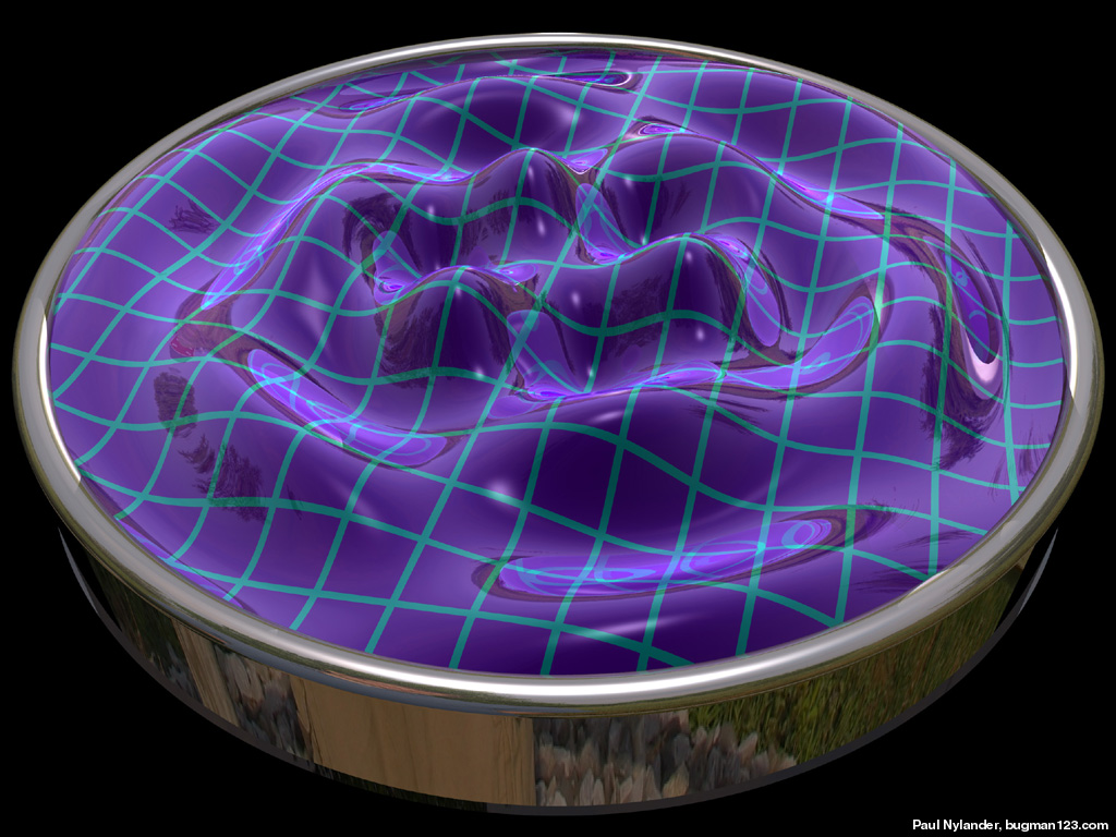
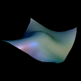
Water Caustics - Mathematica 4.2, POV-Ray 3.1, 4/22/06
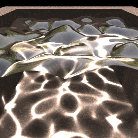

 This water-like surface was generated in Mathematica using frequency filtered random noise, and then it was raytraced in POV-Ray and water caustics were added using Henrik Jensen’s photon mapping technique. The smooth_triangle command was used for phong normal interpolation of the water’s surface.
Links Water Caustics Generator - C++ program by Kjell Andersson, uses Heron’s Formula to calculate the caustics Mathematica simulation - by Daniel Walsh |
Rayleigh Surface Waves - adapted from Daniel Russell's Mathematica code, C++, 11/2/07
 Rayleigh Surface Waves are associated with ocean waves and earthquakes. The following Mathematica code was adapted from Daniel Russell's Rayleigh Surface Waves notebook:
(* runtime: 0.2 second *) omega = 2 Pi; k = 7; nu = 0.33; n = 0.175; xi = Sqrt[(0.5 - nu)/(1 - nu)]; q = k Sqrt[1 - n^2 xi^2]; s = k Sqrt[1 - n^2]; Do[grid = Table[{x + k (Exp[q y] - 2 q s Exp[s y]/(s^2 + k^2)) Sin[omega t - k x], y + q (Exp[q y] - 2 k^2 Exp[s y]/(s^2 + k^2)) Cos[omega t - k x]}, {x, 0, 2, 0.1}, {y, -1, 0, 0.1}]; Show[Graphics[{Map[Line, grid], Map[Line, Transpose[grid]]}, AspectRatio -> Automatic, PlotRange -> {{-0.1, 2.1}, {-1.1, 0.25}}]], {t, 0, 1, 0.05}]; Links Animated Gif - by Daniel Russell Oceanography Waves - webpage by J Floor Anthoni |
Horseshoe Magnets - new version: POV-Ray 3.6.1, 7/15/06
old version: calculated in Mathematica 4.2, rendered in TrueSpace 4.3, 3/9/03
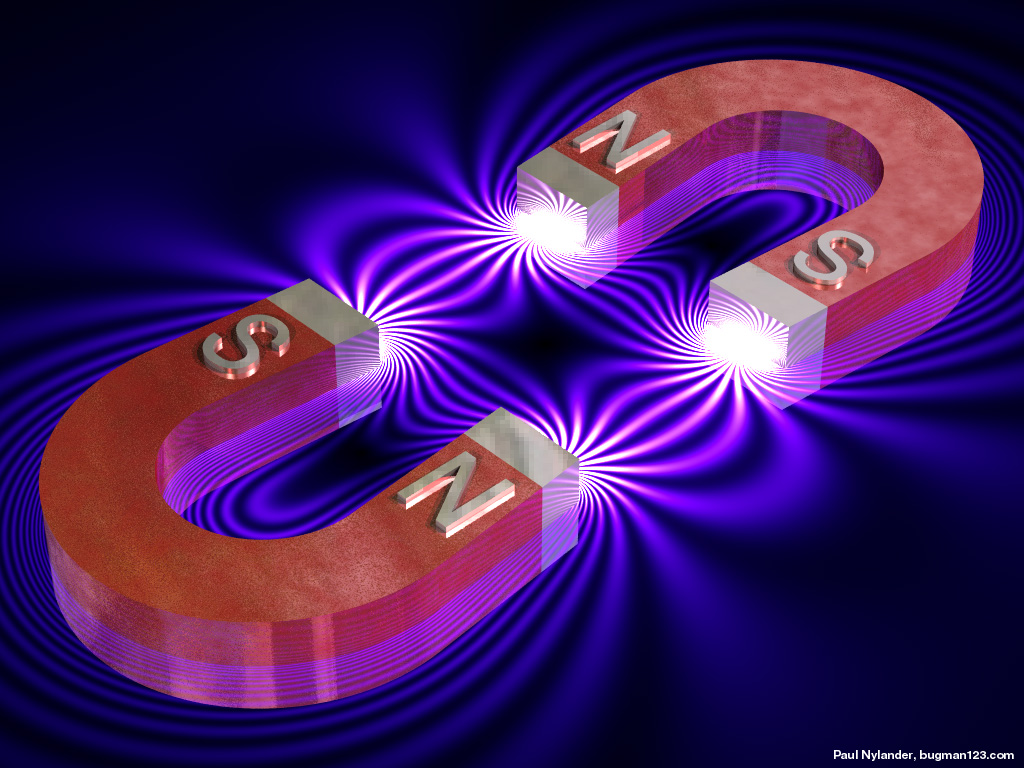
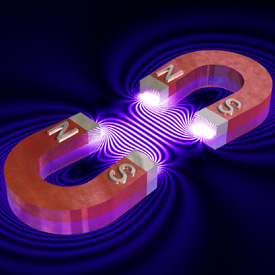
 These magnetic fields were made using the same technique as the solenoid picture.
 |
 Links
LinksLevitron - magnetic levitating top Molecular Magnetism - magnetic levitation of a frog in a Bitter solenoid Gravitator - magnetic levitating sphere Geodynamo Lab - I recently had the opportunity to tour this lab at the University of Maryland Bar Magnet Calculator - JavaScript program Electromagnetic Field in Microwave Oven - interesting discussion by Wenjun Deng (my former roommate) |
Halo Orbit - calculated in Mathematica 4.2, rendered in POV-Ray 3.6.1, 12/1/05
 In 1772, Joseph Lagrange showed that a small satellite moving in the Earth-Moon system can have 5 balance points, called Lagrange points. Here is a small halo orbit around Lagrange point L4. This is interesting because L4 is off to the side, so it looks like the satellite is orbiting nothing! The velocity components have been represented by the third axis and color. Here is some Mathematica code:
(* runtime: 6 seconds *) Clear[x, y, t, p, v]; mu = 0.0123001; x1 = -mu; x2 = 1 - mu; r1 = Sqrt[(x - x1)^2 + y^2]; r2 = Sqrt[(x - x2)^2 + y^2]; {x0, y0} = {x, y} /. Last[NSolve[{-x == -x2(x - x1)/r1^3 + x1(x - x2)/r2^3, -y == -(x2/r1^3 - x1/r2^3) y}, {x, y}]]; JacobianMatrix[p_, q_] := Outer[D, p, q]; vlist = Eigenvectors[JacobianMatrix[{xdot, -x2(x - x1)/r1^3 + x1(x - x2)/r2^3 + 2ydot + x, ydot, -(x2/r1^3 - x1/r2^3)y - 2xdot + y}, {x, xdot, y, ydot}] /. {x -> x0, xdot -> 0, y -> y0, ydot -> 0}]; r1 = Sqrt[(x[t] - x1)^2 + y[t]^2]; r2 = Sqrt[(x[t] - x2)^2 + y[t]^2]; tmax = 355; p0 = {x0, y0, 0, 0} + Re[0.5 vlist[[1]] + vlist[[3]]]/3.84400*^5; p[t_] = {x[t], y[t]} /. NDSolve[{x''[t] - 2y'[t] - x[t] == -x2(x[t] - x1)/r1^3 + x1(x[t] - x2)/r2^3, y''[t] + 2x'[t] - y[t] == -(x2/r1^3 - x1/r2^3)y[t], x[0] == p0[[1]], y[0] == p0[[2]], x'[0] == p0[[3]], y'[0] == p0[[4]]}, {x[t], y[t]}, {t, 0, tmax}, MaxSteps -> 100000, AccuracyGoal -> 10][[1]]; v[t_] = D[p[t], t]; ParametricPlot3D[Append[p[t], v[t][[1]]], {t, 0, tmax}, Compiled -> False, PlotPoints -> 1000, BoxRatios -> {1, 1, 1}, ViewPoint -> {0, 10, 0}] Links Interplanetary Superhighway - by Shane Ross Stable 3-Body Orbits - Java applet by Robert Vanderbei, be sure to see the Ducati 3-Body Orbit |
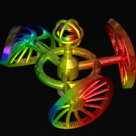
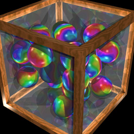
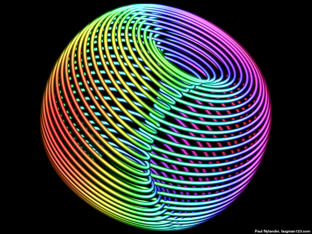
Cross Section of the Quintic Calabi-Yau Manifold - Mathematica 4.2, POV-Ray 3.1, 8/25/08

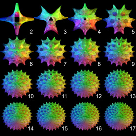
 The left picture shows a 3D cross section of the quintic 6D Calabi-Yau Manifold proposed for String Theory. The right picture shows various degrees of complexity. Click here to download some POV-Ray code for this image. Here is some Mathematica code:
(* runtime: 54 seconds, change n for other degrees of complexity *) n = 5; CalabiYau[z_, k1_, k2_] := Module[{z1 = Exp[2Pi I k1/n]Cosh[z]^(2/n), z2 = Exp[2Pi I k2/n]Sinh[z]^(2/n)}, {Re[z1], Re[z2], Cos[alpha]Im[z1] + Sin[alpha]Im[z2]}]; Do[alpha = (0.25 + t)Pi; Show[Graphics3D[Table[ParametricPlot3D[CalabiYau[x + I y, k1, k2], {x, -1, 1}, {y, 0, Pi/2}, DisplayFunction -> Identity, Compiled ->False][[1]], {k1, 0, n - 1}, {k2, 0, n - 1}], PlotRange -> 1.5{{-1, 1}, {-1, 1}, {-1, 1}}, ViewPoint -> {1, 1, 0}]], {t, 0, 1, 0.1}]; Links The Elegant Universe - 3 hour online mini-series on String Theory by NOVA Calabi-Yau etched in Crystal - by Bathsheba Grossman Calabi-Yau Cross Sections - by Andrew Hanson Equations - Stewart Dickson Math |
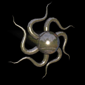
Vibration Mode of a Spherical Membrane - Mathematica 4.2, MathGL3d, 9/28/04
 This is a somewhat exaggerated example of how a spherical balloon might vibrate. Here is some Mathematica code:
(* runtime: 4 seconds *) Y := Re[SphericalHarmonicY[8, 4, theta, phi]]; r := (1 + 0.5Y); ParametricPlot3D[{r Sin[theta] Cos[phi], r Sin[theta] Sin[phi], r Cos[theta], {EdgeForm[], SurfaceColor[Hue[Y]]}}, {theta, 0, Pi}, {phi, 0, 2Pi}, PlotPoints -> 72, Boxed -> False, Axes -> None] Links Click here to read more about spherical harmonics. Spherical Harmonic Lighting - interesting technique for global illumination by Paul Baker |
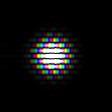
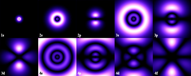
Hydrogen Electron Orbital Probability Distribution Cross-Sections - Mathematica 4.2, 4/30/03
Here are some different shapes that a hydrogen atom can take. These plots are based on the same function as the vibrating balloon (shown above):
P = 4 π r2ψr2ψθ2, ψr = e-ρρlLn-1-l2l+1(ρ), ψθ = Ylm(θ,φ), ρ = 2r/n
|
(* runtime: 10 second *) P[n_, l_, m_, {x_, y_, z_}] := Module[{r = Sqrt[x^2 + y^2 + z^2]}, 4 Pi r^2(Exp[-r/n]r^l LaguerreL[n - 1 - l, 2l + 1, 2 r/n])^2 Abs[SphericalHarmonicY[l, m, ArcCos[z/r], ArcTan[x, y]]]^2]; DensityPlot[P[3, 1, 0, {x, 0, z}], {x, -20, 20}, {z, -20, 20}, Mesh -> False, PlotPoints -> 275, Frame -> False, Compiled -> False] |
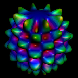
Hydrogen 4f Electron Orbital Probability Distribution
C++ version: 8/10/09; Mathematica version: 8/22/04; animations: C++, POV-Ray 3.6.1, 11/27/05
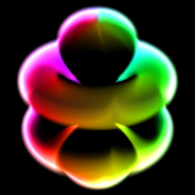
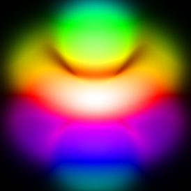

 Here is a 3D view of a hydrogren atom in the 4f state. The left image was made in C++ using a technique described by Krzysztof Marczak to make it volumetric like a cloud of smoke. The right image was made in Mathematica by adding 2D cross-sectional layers. The animations were made in POV-Ray using DF3 density files. The right animation shows what a "12o" orbital might look like.
POV-Ray has a built-in internal function for the 3d orbital: // runtime: 4 seconds camera{location 16*z look_at 0} #declare P=function{internal(53)}; #declare P0=P(0,3,0,0); box{-8,8 pigment{rgbt t} hollow interior{media{emission 0.5 density{function{(P(x,y,z,0)-1.2)/(P0-1.2)} color_map{[0 rgb 0][1 rgb 1]}}}}} Links Atomic Orbital - time-dependant hydrogen atom simulation, by ? Orbital Viewer - Java applet by Paul Falstad HydrogenLab - animations of hydrogen energy transitions |
Zoom Animation - Google Maps API, POV-Ray 3.6.1, 10/29/07
 I made this using Google Maps.
Links Google Sightseeing - discover the world via Google Maps Celestia - impressive free 3D space simulation software by Chris Laurel Celestia Addon Catalogs - Joseph Bolte, Bruckner’s Celestia Page WorldWide Telescope - by Microsoft JTrack 3D - fun satellite tracker Java applet Powers of 10 - Java applet Google Earth - fun program to explore satellite imagery around the globe Earth POV-Ray Code - by James Kuffner Google Maps API Developer's Guide |
Fundamental Modes of Vibration for a Violin-Shaped Membrane - GeoStar 2.8, AutoCAD 2000, 4/21/04
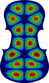
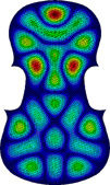
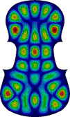 Mode displacement plots of the 19th, 28th, and 45th modes, respectively, from left to right. Click here to see a holographic interferogram of a real violin.
|
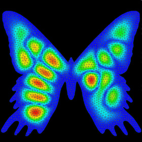 Mode displacement plot of the 18th mode of a Sunset Moth-Shaped Membrane.
|
31st Fundamental Mode of Vibration of a Circular Membrane - Mathematica 4.2, MathGL3d, 11/10/03
 This is an example of how a circular drumhead might vibrate. Click here to see a large animation. Click here to see a rotatable animated version. Here is some Mathematica code:
J3(k43r)cos(3θ) → frequency: f31 = f1k43/k10 = 6.74621 f1 (* runtime: 5 seconds *) Clear[r]; << NumericalMath`BesselZeros`; k = BesselJZeros[3, 4][[4]]; << MathGL3d`OpenGLViewer`; texture = Graphics[{RGBColor[0, 1, 1], Rectangle[{0, 0}, {10, 10}], RGBColor[0.5, 0, 1], Rectangle[{1, 1}, {9, 9}]}]; MVShow3D[ParametricPlot3D[{r Sin[theta], r Cos[theta], 0.25BesselJ[3, k r]Cos[3 theta]}, {r, 0, 1}, {theta, 0, 2Pi}, PlotPoints -> {56, 168}], MVNewScene -> True, MVTexture -> texture, MVTextureMapType -> MVMeshUVMapping, MVScaleTexture -> {14, 42}] Links Vibrating Drumheads - by Jim Swift Cymatics - wave patterns created by sound waves Soap Film Oscillations - interesting old video Oscillating Soap Film - MIT video |
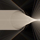
Magnifying Glass - POV-Ray 3.6.1, 3/20/07

 This magnifying glass demonstrates refraction and dispersion. The magnifying glass was created by intersecting two paraboloids.
 |
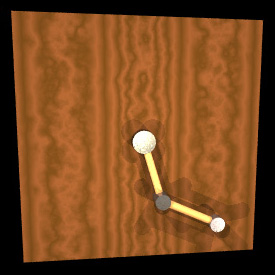
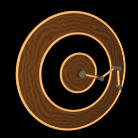
Spherical Pendulum - calculated in Mathematica 4.2, rendered in POV-Ray 3.6.1, 1/10/06
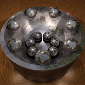
 The spheres in this frictionless bowl move like spherical pendulums. See also my magnetic pendulum fractals.
(* runtime: 0.03 second *) Clear[theta, phi]; g = 9.81; soln = NDSolve[{theta''[t] == (phi'[t]^2Cos[theta[t]] - g)Sin[theta[t]], phi''[t]Tan[theta[t]] == -2phi'[t]theta'[t], theta[0] == Pi/2, phi[0] == 0, theta'[0] == 0, phi'[0] == 2.357}, {theta[t], phi[t]}, {t, 0, 8}][[1]]; ParametricPlot3D[{Sin[theta[t]]Cos[phi[t]], Sin[theta[t]]Sin[phi[t]], -Cos[theta[t]]} /. soln, {t, 0, 8}, Compiled -> False] Here is some Mathematica code to animate it: (* runtime: 0.6 second *) << Graphics`Shapes`; Do[p = {Sin[theta[t]]Cos[phi[t]], Sin[theta[t]]Sin[phi[t]], -Cos[theta[t]]}; Show[Graphics3D[{EdgeForm[], Line[{{0, 0, 0}, p}], TranslateShape[Sphere[0.2, 10, 6], p]}, PlotRange -> 1.2{{-1, 1}, {-1, 1}, {-1, 1}}]], {t, 0, 8, 0.1}]; |
Cloth Simulation - Mathematica 4.2, MathGL3d, 7/11/05
 This cloth is modelled as a net of small springs and masses. The following Mathematica code still needs some improvement:
(* runtime: 2 minutes *) Normalize[p_] := p/Sqrt[p.p]; r = 0.5; n = 13; dx = 2.0/(n - 1); dt = 0.05; g = {0, 0, -0.2}; cloth = Table[{{x, y, r}, {0, 0, 0}}, {y, -1, 1, dx}, {x, -1, 1, dx}]; Do[ Show[Graphics3D[{EdgeForm[], Map[Polygon[Flatten[#, 1][[{1,2, 4, 3}, 1]]] &, Partition[cloth, {2, 2}, 1], {2}]}, PlotRange -> {{-1,1}, {-1, 1}, {-1, 1}}]]; Do[cloth = Table[{p1, v1} = cloth[[i, j]]; If[(i == 1 || i == n) && (j == 1 || j == n), {p1, v1},v2 = v1 + g dt; Do[i2 = i + di; j2 = j + dj; If[! (i2 == i && j2 == j) && 0 < i2 <= n && 0 < j2 <= n, L0 = dx Sqrt[(j2 - j)^2 + (i2 - i)^2]; p2 = cloth[[i2, j2, 1]]; L = Sqrt[(p2 - p1).(p2 - p1)]; v2 += (L/L0 - 1)Normalize[p2 - p1]dt], {di, -2, 2}, {dj, -2, 2}]; v2 *= 0.9; {p1 + (v1 + v2) dt/2,v2}], {i, 1, n}, {j, 1, n}], {25}], {10}]; Links OpenGL program - by Paul Baker Cloth Animations - by Ron Fedkiw, Robert Bridson, et al. Cloth and Fur Energy Functions - Pixar presentation |
Fraunhofer Diffraction of Light Through a Circular Aperature - Mathematica 4.2, 8/24/04
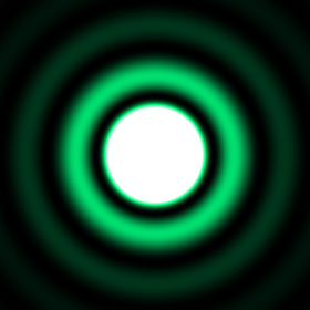
 When parallel light passes through a small hole and a shadow is cast on a wall, there will be small diffraction ridges along the edge of the shadow. These ridges become smaller when the frequency of the light is increased. See also my single slit diffraction of a green laser. Here is some Mathematica code:
(* runtime: 16 seconds *) Clear[i]; lambda = 500*^-9; k = 2Pi/lambda; a = 80*^-6; i[rho_] := (2Pi a BesselJ[1, k a rho]/(k rho))^2; DensityPlot[i[Sqrt[u^2 + v^2]], {u, -0.01, 0.01}, {v, -0.01, 0.01}, Mesh -> False, PlotPoints -> 275, Frame -> False] |
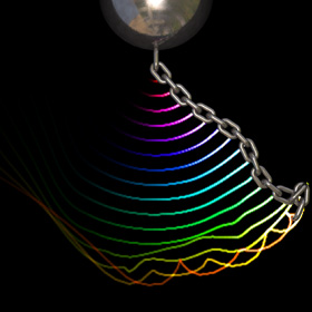
Vibrating String with Damping - calculated in Mathematica 4.2, rendered in POV-Ray 3.6.1, 1/27/06
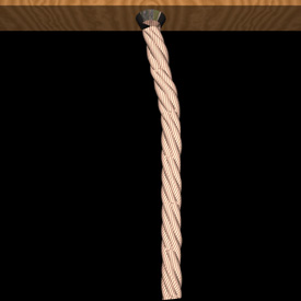

 This analytical solution for a vibrating string was solved using the method of separation of variables assuming small linear perturbations. The rope was drawn using Mike Williams’ rope macro. Here is some Mathematica code: (* runtime: 2 seconds *) c = 4; L = 1; h = 0.1; b = Pi; k := (n - 0.5)Pi/L; omega := Sqrt[(c k)^2 - (0.5b)^2]; Do[Plot[Evaluate[Sum[(6h/k^2)Sin[k/3] Exp[-0.5b t](Cos[omega t] + (0.5b/omega) Sin[omega t])Sin[k x], {n, 1, 10}]], {x, 0,L}, PlotRange -> {{0, L}, {-h, h}}, AspectRatio -> Automatic], {t, 0, 1.5, 0.025}]; |
Wave Interference - Mathematica 4.2, 8/24/04
 This interference pattern is the superposition of two wave sources, such as light passing through two narrow slits. Here is some Mathematica code:
(* runtime: 9 seconds *) Do[DensityPlot[Sin[2Pi(Sqrt[x^2 + (y - 3)^2] + t)] + Sin[2Pi(Sqrt[x^2 + (y + 3)^2] + t)], {x, 0, 16}, {y, -8, 8}, PlotPoints -> 275, Mesh -> False, Frame -> False], {t, 0, 1, 0.1}]; |
Physics Theory Links
First Time Machine - interesing Discovery video about making a time machine using lasers
Physics Lectures - free videos by Walter Lewin at MIT
HyperPhysics - Georgia State University
See also my Physics Experiments links.