


Hypercomplex numbers are similar to the usual 2D complex numbers, except they can be extended to 3 dimensions or more. When you use hypercomplex numbers to generate fractals, you can create some interesting looking 3D fractals.
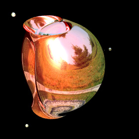
Quadratic 3D Mandelbulb Set - C++, 7/3/09
 This hypercomplex fractal is based on Daniel White's creative formula for squaring a 3D hypercomplex number ("triplex") by applying two consecutive rotations using a spherical coordinate system:
{x,y,z}2 = r2{cos(θ)cos(φ),sin(θ)cos(φ),-sin(φ)} r2=x2+y2+z2, θ=2atan2(y,x), φ=2sin-1(z/r) This formula can also be expressed in non-trigonometric form: 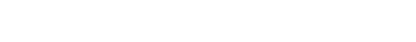 One drawback about this formula is that it doesn't allow you to define a very consistent set of operators (click here for a more consistent formula). However, I think it creates the best looking quadratic 3D Mandelbrot set so far. Here is some Mathematica code demonstrating a simple way to render this 3D fractal as a depth map by slowly marching tiny cubes (voxels) toward the boundary: (* runtime: 1.7 minutes, increase n for higher resolution *) n = 100; norm[x_] := x.x; TriplexSquare[{x_, y_, z_}] := If[x == y == 0, {-z^2, 0, 0}, Module[{a = 1 - z^2/(x^2 + y^2)}, {(x^2 - y^2)a, 2 x y a, -2 z Sqrt[x^2 + y^2]}]]; Mandelbulb[c_] := Module[{p = {0,0, 0}, i = 0}, While[i < 24 && norm[p] < 4, p = TriplexSquare[p] + c; i++]; i]; image = Table[z = 1.5; While[z >= -0.1 && Mandelbulb[{x, y, z}] < 24, z -= 3/n]; z, {y, -1.5, 1.5, 3/n}, {x, -2, 1, 3/n}]; ListDensityPlot[image, Mesh -> False, Frame -> False, PlotRange -> {-0.1, 1.5}] Here is some inefficient code demonstrating how you can render this isosurface in POV-Ray using recursive functions: // runtime: 4.5 minutes camera{location <-2.5,5,5> look_at <-0.5,0,0.25> up z sky z angle 25} light_source{20*z,1} #declare f=function(i,x,y,z,xc,yc,zc) {select(i>0 & x*x+y*y+z*z<4, 0, sqrt(x*x+y*y+z*z), f(i-1,(x*x-y*y)*(1-z*z/(x*x+y*y))+xc,2*x*y*(1-z*z/(x*x+y*y))+yc,-2*z*sqrt(x*x+y*y)+zc,xc,yc,zc))}; isosurface{function{f(24,x,y,z,x,y,z)} threshold 2 max_gradient 10 contained_by{sphere{<-0.5,0,0>,2}} pigment{rgb 1}} When I first set out to render these fractals, I couldn't find any software that could ray-trace iterated isosurfaces so I had to write my own C++ program for it. At first, this seemed like a daunting task, but with some help from Thomas Ludwig, and some useful links, it turned out not to be as difficult as I thought. I made the top image using a volumetric technique described by Krzysztof Marczak. This image was precomputed using a volume of 1.4 billion voxels. I made the other images using James Kajiya's path tracing method for Global Illumination (GI). This method uses Monte Carlo integration to solve the rendering equation. Links Mandelbrot 3D, cut away view - by Krzysztof Marczak metallic rendering - by Thomas Ludwig 3D Mandelbrot, Coral Rift - rendering with global illumination, by Thomas Ludwig, see also the discussion on Fractal Forums inside view - by Krzysztof Marczak animation - by Bib animations - uses different powers for each rotation, by Bill Rood Global Illumination and Participating Media Links smallpt - Global Illumination in 99 lines of C++, by Kevin Beason MiniLight - simple global illumination renderer Subsurface Scattering - Wikipedia Subsurface Scattering - papers by Henrik Jensen, explains how to simulate subsurface scattering using photon mapping |

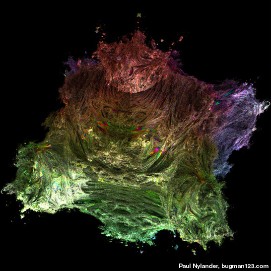
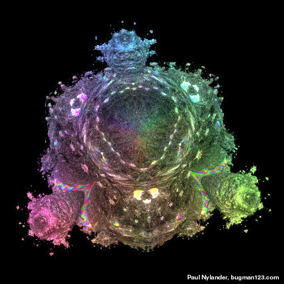
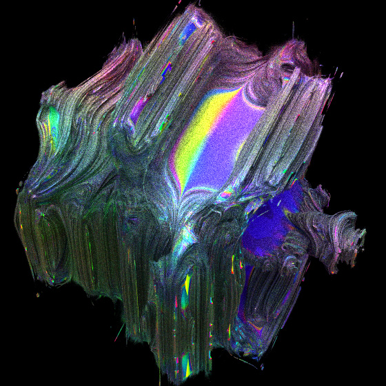
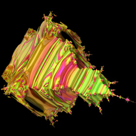
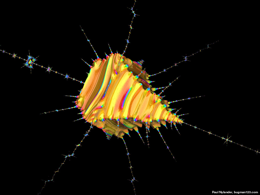
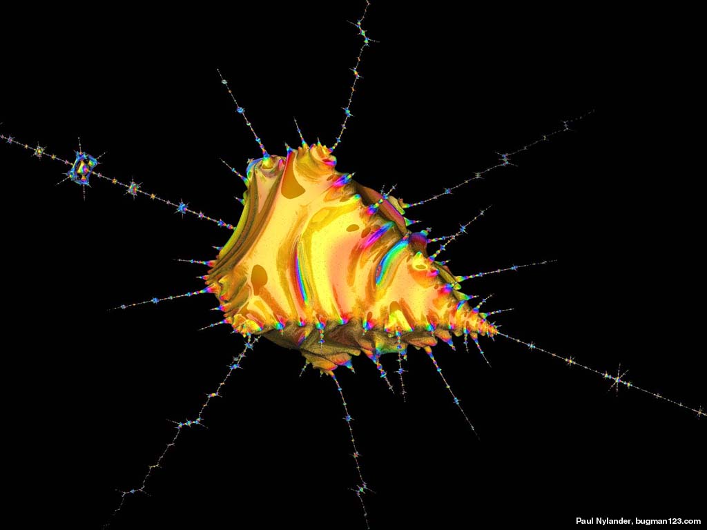
3D Power Mandelbulb Set - C++, 8/20/09
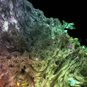
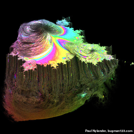
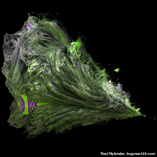
 Here is my first rendering of an 8th order Mandelbulb set, based on the following generalized variation of Daniel White's original squarring formula:
{x,y,z}n = rn{cos(θ)cos(φ),sin(θ)cos(φ),-sin(φ)} r=sqrt(x2+y2+z2), θ=n atan2(y,x), φ=n sin-1(z/r) I originally posted this image on 8/30/09. Daniel White was very excited when he first saw this rendering because it has significantly finer 3D details than the quadratic version. He wrote a beautiful article about it, calling it the "Mandelbulb" (I believe it was Rudy Rucker who coined the name). The Mandelbulb rapidly grew in popularity, and it was presented in many popular articles including Slashdot, New Scientist magazine, Wikipedia, and Science & Vie magazine. Here is some Mathematica code: (* runtime: 1.4 minutes, increase n for higher resolution *) n = 100; norm[x_] := x.x; TriplexPow[{x_, y_, z_}, n_] := If[x == y == 0.0, 0.0, Module[{r = Sqrt[x^2 + y^2 + z^2], theta = n ArcTan[x, y], phi}, phi = n ArcSin[z/r]; r^n{Cos[theta]Cos[phi], Sin[theta]Cos[phi], -Sin[phi]}]]; Mandelbulb[c_] := Module[{p = {0, 0, 0}, i = 0}, While[i < 24 && norm[p] < 4, p = TriplexPow[p, 8] + c; i++]; i]; image = Table[z = 1.1; While[z >= -0.1 && Mandelbulb[{x, y, z}] < 24, z -= 2.2/n]; z, {y, -1.1, 1.1, 2.2/n}, {x, -1.1, 1.1, 2.2/n}]; ListDensityPlot[image, Mesh -> False, Frame -> False, PlotRange -> {-0.1, 1.1}] We can increase the speed / accuracy and emphasize the boundaries using distance estimation: (* runtime: 1.7 minute *) abs[x_] := Sqrt[x.x]; TriplexMult[{x1_, y1_, z1_}, {x2_, y2_, z2_}] := Module[{r1 = Sqrt[x1^2 + y1^2], r2 = Sqrt[x2^2 + y2^2], a}, a = 1 - z1 z2/(r1 r2); {a(x1 x2 - y1 y2), a(x2 y1 + x1 y2), -(r2 z1 + r1 z2)}]; DistanceEstimate[c_, n_] :=Module[{p = {0, 0, 0}, dp = {1, 0, 0}, r, dr = 1, i = 0, loop = True}, While[loop, p = TriplexPow[p, n] + c; r = abs[p]; i++; loop = (i < 24 && r < 2); If[loop, dp = n TriplexMult[dp, TriplexPow[p, n - 1]] + {1, 0, 0}; dr = abs[dp]]]; 2 r Log[r]/dr/4]; n = 100; image = Table[z = d = 1.1; While[d > 0.001 && z >= -0.1, d = DistanceEstimate[{x, y, z}, 8]; z -=d]; z, {y, -1.1, 1.1, 2.2/n}, {x, -1.1, 1.1, 2.2/n}]; ListDensityPlot[image,Mesh -> False, Frame -> False, PlotRange -> {-0.1, 1.1}] Here is some inefficient code demonstrating how you can render this isosurface in POV-Ray using recursive functions: // runtime: 28 minutes camera{location <1.75,4,5.5> look_at 0 up z sky z angle 25} light_source{20*z,1} #declare n=8; #declare f=function(i,x,y,z,xc,yc,zc) {select(i>0 & x*x+y*y+z*z<4, 0, sqrt(x*x+y*y+z*z),f(i-1,pow(x*x+y*y+z*z,n/2)*cos(n*atan2(y,x))*cos(n*atan2(z,sqrt(x*x+y*y)))+xc,pow(x*x+y*y+z*z,n/2)*sin(n*atan2(y,x))*cos(n*atan2(z,sqrt(x*x+y*y)))+yc,-pow(x*x+y*y+z*z,n/2)*sin(n*atan2(z,sqrt(x*x+y*y)))+zc,xc,yc,zc))}; isosurface{function{f(24,0,0,0,x,y,z)} threshold 2 max_gradient 1000 contained_by{sphere{0,1.5}} pigment{rgb 1}} I posted some non-trigonometric expansions for this formula here and here. The above animation was created by adding a phase shift to φ. |

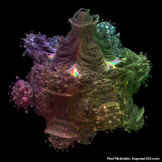

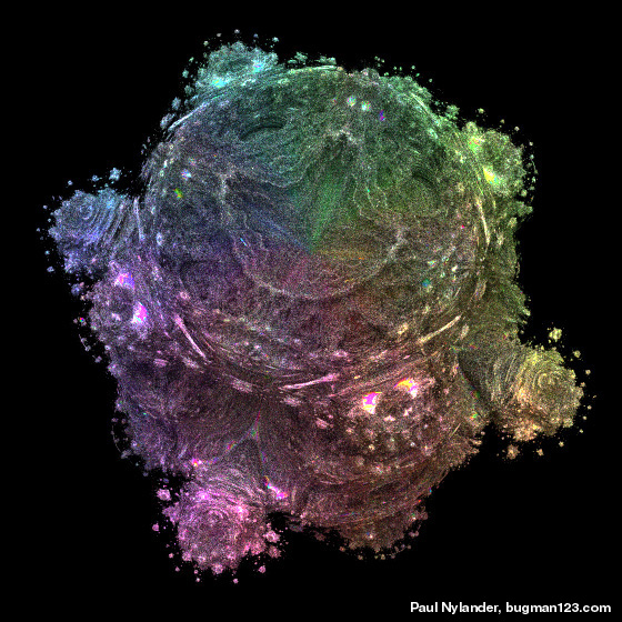
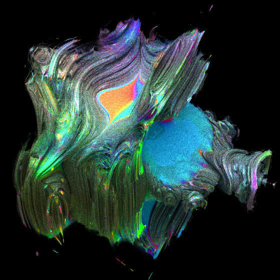
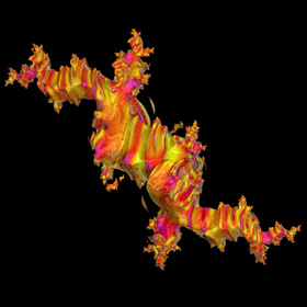
Positive Z-Component Variation of the 3D Mandelbulb Set - C++, 10/3/09
 One strange thing about the previous formula is that it gives {x, y, z}1 = {x, y, -z}. Here is a more consistent formula without the negative sign in front of the z-component:
{x,y,z}n = rn{cos(θ)cos(φ),sin(θ)cos(φ),sin(φ)}, r=sqrt(x2+y2+z2), θ=n atan2(y,x), φ=n sin-1(z/r) Using this formula, we have been able to come up with definitions for multiplication, division, powers, roots, exponentials, logarithms, and trigonometric functions. It should be noted that the multiplication operator is commutative but not associative. I also posted some non-trigonometric expansions for the power formula here. One drawback about this formula is that it gives a flat looking quadratic Mandelbrot set. Here is the non-trigonometric form of the multiplication operator:  Here is the non-trigonometric form of the division operator:  |
|

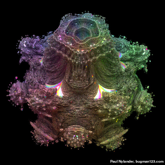
3D Juliabulb Set - C++, 7/28/09
 The left image is a 3D Julia set based on Daniel White's squarring formula for squaring a 3D hypercomplex number (or "Juliabulb" set). The right image is the 4th order variation.
Links JuliaBulb morph - animation, by Bib morphing Juliabulb animation - by I�igo Quilez Juliabulb Sets - 4th order, 3rd order, 3rd order cave, by Krzysztof Marczak Juliaberry - Juliabulb set, by Tom Beddard True 3D Julia - 4th order Juliabulb set by David Makin The Honeycomb - 10th order Juliabulb set, by David Makin Thornton Julia Triplex - animation based on Garth Thornton's formula for squaring a 3D hypercomplex number, by David Makin, see also this |
|
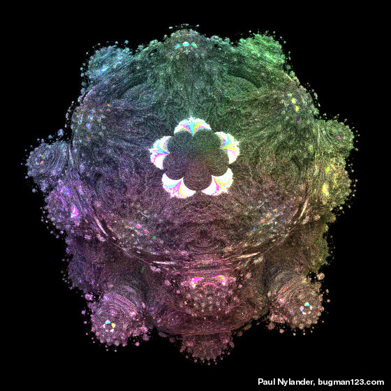
Lambdabulb 3D Juliabulb Set - C++, 11/25/09
 An endless variety of 3D Mandelbulb and Juliabulb sets are possible using triplex numbers. For example, here is a "Lambdabulb" fractal. This is actually a Juliabulb set that is based on a unique formula suggested by Ron Barnett. Here is some Mathematica code:
(* runtime: 2 minutes, increase n for higher resolution *) TriplexPow[{x_, y_, z_}, n_] := Module[{r = Sqrt[x^2 + y^2 + z^2], theta = n ArcTan[x, y], phi}, phi = n ArcSin[z/r]; r^n{Cos[theta]Cos[phi], Sin[theta]Cos[phi], Sin[phi]}]; TriplexMult[{x1_, y1_, z1_}, {x2_, y2_, z2_}] := Module[{r1 = Sqrt[x1^2 + y1^2], r2 = Sqrt[x2^2 + y2^2], a}, a = 1 -z1 z2/(r1 r2); {a(x1 x2 - y1 y2), a(x2 y1 + x1 y2), r2 z1 + r1 z2}]; c = {1.0625, 0.2375, 0.0}; n = 100; norm[x_] := x.x; Lambdabulb[c_] := Module[{p = c, i = 0}, While[i < 40 && norm[p] < 4, p = TriplexMult[c, p - TriplexPow[p, 4]]; i++]; i]; image = Table[z = 1.2; While[z >= 0 && Lambdabulb[{x, y, z}] < 40, z -= 2.4/n]; z, {y, -1.2, 1.2, 2.4/n}, {x, -1.2, 1.2, 2.4/n}]; ListDensityPlot[image, Mesh -> False, Frame -> False, PlotRange -> {0, 1.2}] |
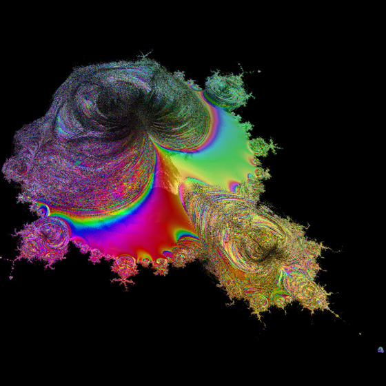
3D Mandelbrot / Mandelbar Set - C++, 7/5/09
 {x,y,z}2 = {x2-y2-z2, 2xy, -2xz}
This method combines the Mandelbrot set with the Mandelbar set (Tricorn). I think Eric Baird was the first to suggest this formula. The right picture is a zoom of the first miniature Mandelbrot set. I think it looks like a space ship with some sort of radar gun. Unfortunately, Julia sets created using this method look the same as quaternion Julia sets. Here is some Mathematica code: (* runtime: 3.2 minutes, increase n for higher resolution *) n = 100; norm[x_] := x.x; TricornSquare[{x_, y_, z_}] := {x^2 - y^2 - z^2, 2x y, -2x z}; Mandelbrot[c_] := Module[{p = {0, 0, 0}, i = 0}, While[i < 20 && norm[p] < 4, p = TricornSquare[p] + c; i++]; i]; image = Table[y = 0.04; While[y > -0.02 && Mandelbrot[{x, y, z}] < 20, y -= 0.08/n]; y, {z, -0.04, 0.04, 0.08/n}, {x, -1.8, -1.72, 0.08/n}]; ListDensityPlot[image, Mesh -> False, Frame -> False, PlotRange -> {-0.02, 0.04}] Here is some inefficient code demonstrating how you can render this in POV-Ray: // runtime: 4 minutes camera{location <-3.5,5,4> look_at <-0.5,0,0.4> up z sky z angle 25} light_source{20*z,1} #declare f=function(i,x,y,z,xc,yc,zc) {select(i>0 & x*x+y*y+z*z<4, 0, sqrt(x*x+y*y+z*z), f(i-1,x*x-y*y-z*z+xc,2*x*y+yc,-2*x*z+zc,xc,yc,zc))}; isosurface{function{f(24,x,y,z,x,y,z)} threshold 2 max_gradient 25 contained_by{sphere{<-0.5,0,0>,2}} pigment{rgb 1}} |


3D Mandelbrot Set Pickover Stalks - C++, 8/18/09

 Pickover stalks are 2D fractals, composed of cross-shaped orbit traps invented by Clifford Pickover. These images were created by extending this concept into 3 dimensions. The right image has helical orbit traps wrapped around the Pickover stalks for added effect. See also my 2D Pickover stalks fractal. Here is some Mathematica code:
(* runtime: 1.5 minutes, increase n for higher resolution *) n = 100; norm[x_] := x.x; TricornSquare[{x_, y_, z_}] := {x^2 - y^2 - z^2, 2x y, -2x z}; OrbitTrap[{x_, y_, z_}] := 1.0 - Min[x^2 + y^2, x^2 + z^2, y^2 + z^2]/0.3^2; Mandelbrot[c_] := Module[{p = {0, 0, 0},i = 0}, While[i < 100 && norm[p] < 4 && (i < 2 || OrbitTrap[p] < 0.0), p = TricornSquare[p] + c; i++]; OrbitTrap[p]]; image = Table[z = 1.5; While[z > -1.5 && Mandelbrot[{x, y, z}] < 0.0, z -= 3/n]; z, {y, -1.5, 1.5, 3/n}, {x, -2.0, 1.0, 3/n}]; ListDensityPlot[image, Mesh -> False, Frame -> False, PlotRange -> All] Links 3D Pickover Stalks - by David Makin 3D Orbit Traps - by I�igo Quilez |


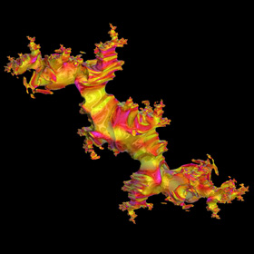
 Here are some Pickover stalks using other 3D Mandelbrot formulas.
 |
4D Quaternion Mandelbrot ("Mandelquat") Set - C++, 7/7/09
 {x,y,z,w}2 = {x2-y2-z2-w2, 2xy, 2xz, 2xw}
Quaternions are 4D hypercomplex numbers, discovered in 1843 by Sir William Rowan Hamilton. They are mathematically elegant, but unfortunately, they produce rather boring looking axisymmetric results when used to calculate the 3D Mandelbrot set. The image in the middle is a zoom of the first miniature Mandelbrot set and the image on the far right shows the 8th order variation of this fractal. Link: Quat Minibrot - by David Makin |
 Here are the orbits of the quaternion Mandelbrot set. This image was created by simply revolving the 2D Mandelbrot orbits.
 |
4D Quaternion Julia Set - Mathematica 4.2: 7/9/04, POV-Ray 3.1: 8/5/04

 This used to be the most popular method for creating hypercomplex fractals. Here is some Mathematica code:
(* runtime: 1.5 minutes *) n = 100; dx = 3/n; c = {-0.2, 0.8, 0, 0}; norm[q_] := q.q; QuatSquare[{x_, y_, z_, w_}] := {x^2 - y^2 - z^2 - w^2, 2 x y, 2 x z, 2 x w}; Julia[q0_] := Module[{q = q0, i = 0}, While[i < 12 && norm[q] < 4, q = QuatSquare[q] + c; i++]; i]; image = Table[z = 1.5; While[z > -1.5 && Julia[{x, y, z, 0}] < 12, z -= 3/n]; z, {y, -1.5, 1.5, dx}, {x, -1.5, 1.5, dx}]; ListDensityPlot[image, Mesh -> False, Frame -> False] We can use fast Phong shading to make it look 3D: (* runtime: 0.3 second *) Normalize[x_] := x/Sqrt[x.x]; ListDensityPlot[Table[x = (j - 1) dx - 1.5; y = (i - 1) dx - 1.5; z = image[[i, j]]; normal = Normalize[{(image[[i, j + 1]] - image[[i, j - 1]])z, (image[[i + 1, j]] - image[[i - 1, j]]) z, 2dx}]; L = {1, 1, 0} - {x, y, z}; reflect = Normalize[2(normal.L)normal - L]; -(normal.Normalize[L] + reflect[[3]]), {i, 2, n}, {j, 2, n}],Mesh -> False, Frame -> False] POV-Ray has an efficient algorithm for ray tracing quaternion Julia sets: // runtime: 8 seconds camera{location <1,1,-2> look_at 0} light_source{<1.5,1.5,-1.5>,1} julia_fractal{<-0.2,0.8,0,0> quaternion sqr max_iteration 12 precision 400 pigment{rgb 1}} Links Ray Tracing Quaternion Julia Sets on the GPU - by Keenan Crane, uses Graphics Processing Unit (GPU) for fast calculations, includes source code, see also his explanation Hypercomplex Iterations - nice pictures Quaternion Julia Sets - multiple isosurfaces at varying iteration depths, by Gert Buschmann YouTube Video - by John Hart real time ray tracer - ported from Keenan Crane's program by Tom Beddard |
Inverse 4D Quaternion Julia Set - C++ version: 9/15/09; POV-Ray, version: 7/4/06; Mathematica version: 7/18/04


 Here is the 4D quaternion Julia set using the inverse Julia set method. The 4th dimension has been color-coded. This method is much faster, but some regions are faint because they attract much slower. The left image contains 2 billion points and the right image contains 500 million tiny spheres. See also my POV-Ray code and rotatable 3D version. Here is some Mathematica code:
(* runtime: 5 seconds *) Sqrt2[q_] := Module[{r = Sqrt[Plus @@ Map[#^2 &, q]], a, b}, a = Sqrt[(q[[1]] + r)/2]; b = (r - q[[1]]) a/(q[[2]]^2 + q[[3]]^2 + q[[4]]^2); {a, b q[[2]], b q[[3]], b q[[4]]}]; QInverse[qlist_] := Flatten[Map[Module[{q = Sqrt2[# - c]}, {q, -q}] &, qlist], 1]; c = {-0.2, 0.8, 0, 0}; qlist = {{1.0, 1.0, 1.0, 1.0}}; Do[qlist = QInverse[qlist], {12}]; Show[Graphics3D[{PointSize[0.005], {Hue[#[[4]]], Point[Delete[#, 4]]} & /@ qlist}, Boxed -> False, Background -> RGBColor[0, 0, 0]]] Links QJulia - inverse quaternion Julia set program by Chris Laurel Quaternion Julia Crystal - laser-etched cube by Bathsheba Grossman |
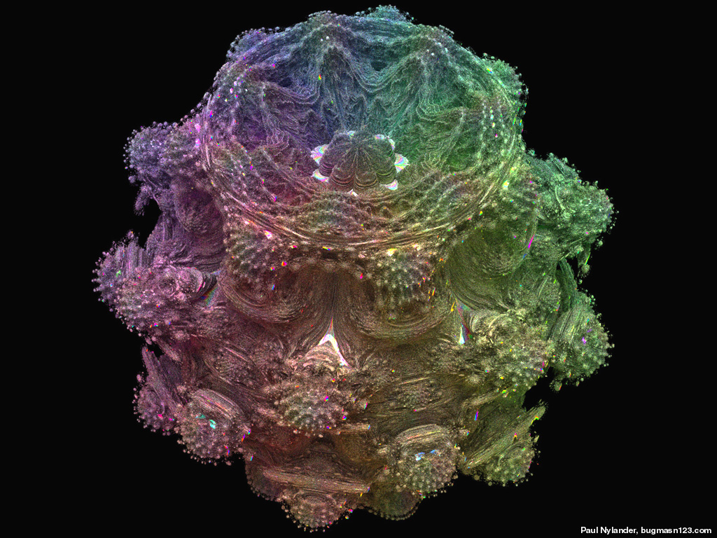
Mandelbox - 2/22/11
|
The Mandelbox fractal is based on an unusual formula originally proposed by Tom Lowe, inspired from the Mandelbulb. Technically, I don't think you can call this a "hypercomplex" fractal, but it seems to exhibit a greater variety of character than the Mandelbulb and has rapidly grown in popularity among fractal artists. Here is some Mathematica code: (* runtime: 3.5 minutes *) n = 100; scale = 2; r0 = 0.5; f = 1; norm[x_] := x.x; BoxFold[p_] := Map[If[# > 1, 2 - #, If[# < -1, -2 - #, #]] &, p]; BallFold[r0_, p_] := Module[{r = Sqrt[norm[p]]}, p/If[r < r0,r0, If[r < 1, r, 1]]^2]; MandelBox[c_] := Module[{p = {0, 0, 0}, i = 0}, While[i < 24 && norm[p] < 4,p = scale BallFold[r0, f BoxFold[p]] + c; i++]; i]; image = Table[z = 1.0; While[z >= 0 && MandelBox[{x, y, z}] < 3,z -= 1/n]; z, {y, -1, 1, 2/n}, {x, -1, 1, 2/n}]; ListDensityPlot[image, Mesh -> False, Frame -> False, PlotRange -> {-0.1, 1}] Links Mandelbox Trip - extremely popular animation by Krzysztof Marczak Happy Birthday Mandelbox! - showcase of works by various artists on Fractal Forums Mandelbox - French article in Images of Mathematics, by Jos Leys Could Be Trouble - impressive images by Hal Tenny Fractal Wasp Troll - impressive image by Johan Andersson Boxplorer - simple program to zoom into the Mandelbox in real time, by Andy Deck The Last Tree - an interesting example of a lone tree, by stoni Untitled - by Florian Sanwald |
Inverse 3D Juliabulb Set - C++, 9/21/09


 These 3D Juliabulb sets were calculated using the inverse Julia set method. In order to implement this method, I had to find the square root of Daniel White's squarring formula. The left image contains 2 billion tiny spheres and the right image contains points. This square root formula has 4 roots, so the total number of points increases by a factor of 4 after each iteration. The following Mathematica code is written for ease of understanding and is not intended to be efficient:
(* runtime: 3 seconds *) TriplexSqrt[{x_, y_, z_}, sign1_, sign2_] := Module[{r = Sqrt[x^2 + y^2 + z^2], a, b, c,d}, a = sign1 Sqrt[y^2 + x^2 (2 + z^2/(x^2 + y^2)) - 2 x r]; b = sign2 Sqrt[r - x - a]/2; c = y^4 + x^2(y^2 - z^2); d = a (x (r + x) + y^2); {b ((x y^2 - d)(x^2 + y^2) - x^3 z^2)/(y c), b, -z/Sqrt[2(r - d(x^2 + y^2)/c)]}]; c = {-0.2, 0.8, 0}; plist = {{1.0, 1.0, 1.0}, {-1.0, -1.0, -1.0}}; Do[plist = Flatten[Map[{TriplexSqrt[# - c, 1, 1], TriplexSqrt[# - c, -1, 1], TriplexSqrt[# - c, 1, -1], TriplexSqrt[# - c, -1, -1]} &, plist], 1], {6}]; Show[Graphics3D[{PointSize[0.005], Point /@ plist}, Boxed -> False, ViewPoint -> {0, 10, 0}]] |
 Here is a 4th order inverse Juliabulb set with 600 million spheres. The triplex raised to the 4th power has 16 unique valid roots. Garth Thornton was the first person to point out that, in general, the triplex raised to the nth power has n2 unique valid roots. I posted a formula for all integer powers here.
There are a variety of Modified Inverse Iteration Methods (MIIM) which can be used to speed up the calculation by pruning dense branches of the tree. One such method is to prune branches when the map becomes contractive (the cumulative derivative becomes large). Here is some Mathematica code: (* runtime: 3 seconds *) norm[x_] := x.x; TriplexPow[{x_, y_, z_}, n_] := Module[{r = Sqrt[x^2 + y^2 + z^2], theta = n ArcTan[x, y], phi},phi = n ArcSin[z/r]; r^n{Cos[theta]Cos[phi], Sin[theta]Cos[phi], Sin[phi]}]; TriplexRoot[{x_, y_, z_}, n_, ktheta_, kphi_] := Module[{dk = If[Mod[n, 2] == 0 && Abs[n] < 4kphi + If[z < 0, 0, 1] <= 3Abs[n], Sign[z]If[Mod[n, 4] == 0, -1, 1], 0], r = Sqrt[x^2 + y^2 + z^2],theta, phi}, theta = (ArcTan[x, y] + (2ktheta + dk)Pi)/n; phi = (ArcSin[z/r] + (2kphi - dk)Pi)/n; r^(1/n){Cos[theta] Cos[phi], Sin[theta]Cos[phi], Sin[phi]}]; c = {-0.2, 0.8, 0}; plist = {}; dpmax = 1.0*^6; imax = 100; p = Table[{1.0, 1.0, 1.0}, {imax}]; dp = Table[1, {imax}]; roots = Table[0, {imax}]; i = 2; power = 4; nroot = power^2; While[i > 1 && Length[plist] < 5000, p[[i]] = TriplexRoot[p[[i - 1]] - c, power, Mod[roots[[i]], power], Floor[roots[[i]]/power]]; dp[[i]] = Abs[power]Sqrt[norm[TriplexPow[p[[i]], power - 1]]]dp[[i - 1]]; plist = Append[plist, p[[i]]]; prune = (i == imax || dp[[i]] > dpmax); If[prune, While[i > 1 && roots[[i]] == nroot - 1, roots[[i]] = 0; i--]; roots[[i]]++, i++; roots[[i]] = 0]]; Show[Graphics3D[Point /@ plist]] |
3D Glynn Juliabulb Set - C++, 11/17/09
 Here is a 3D variation of the Glynn Julia set, based on my modified version of Daniel White's squarring formula for raising a 3D hypercomplex number ("triplex") to the power of 1.5. This was rendered as a point cloud with many tiny spheres using the Modified Inverse Iteration Method (MIIM). Finding all the unique valid roots was a challenge. In general, I found that there are at least 2 roots when x < 0 and at least one root when x > 0. But there is also a strange conic section region containing 3 roots when z2 > x2 + y2. It should also be noted that convergence is very sensitive to the initial seed value. I found the best results when the seed value is inside one of the cones of the conic section. But this only finds one half of the overall fractal. You can find the other half by placing the seed in the other cone, but I preferred to leave this part out, because it gives a nice cross-section so you can see inside the fractal. See also my 2D Glynn Julia sets. Here is some Mathematica code:
(* runtime: 15 seconds *) power = 1.5; norm[x_] := x.x; TriplexPow[{x_, y_, z_}, n_] := Module[{r = Sqrt[x^2 + y^2 + z^2], theta = n ArcTan[x, y], phi},phi = n ArcSin[z/r]; r^n{Cos[theta] Cos[phi], Sin[theta]Cos[phi], Sin[phi]}]; NumRootsGlynn[{x_, y_, z_}] := If[z^2 > x^2 + y^2, 3, If[x < 0, 2, 1]]; TriplexRootGlynn[{x_, y_, z_}, k_] := Module[{r = Sqrt[x^2 + y^2 + z^2], ktheta, kphi, theta, phi}, {ktheta, kphi} = If[k == 0, {0, 0}, If[z^2 > x^2 + y^2, If[k == 1, If[x <0 && y < 0, {2, 0}, {0.5, If[z > 0, 0.5, 2.5]}], If[x < 0 && y > 0, {1, 0}, {2.5, If[z > 0, 0.5, 2.5]}]], {If[y < 0, 2, 1], 0}]]; theta = (ArcTan[x, y] + ktheta Pi)/power; phi = (ArcSin[z/r] +kphi Pi)/power; r^(1/power){Cos[theta] Cos[phi], Sin[theta]Cos[phi], Sin[phi]}]; c = {-0.2, 0, 0}; imax = 100; dpmax = 50.0; p = Table[{-0.61, 0.0, -0.42}, {imax}]; dp = Table[1, {imax}]; roots = Table[0, {imax}]; plist = {}; i = 2; While[i > 1 && Length[plist] < 10000, p[[i]] = TriplexRootGlynn[p[[i - 1]] - c, roots[[i]]]; dp[[i]] = Abs[power]Sqrt[norm[TriplexPow[p[[i]], power - 1]]]dp[[i - 1]];plist = Append[plist, p[[i]]]; prune = (i == imax || dp[[i]] > dpmax); If[prune, While[i > 1 && roots[[i]] == NumRootsGlynn[p[[i - 1]] - c] - 1, roots[[i]] = 0; i--]; roots[[i]]++, i++; roots[[i]] = 0]]; Show[Graphics3D[{PointSize[0.005], Point /@ plist}]] Links Glynn Juliabulb - interesting variation based on the cosine power formula, looks like a "weaved" clam shell, by Jos Leys Tripcove Fractal - another interesting variation probably based on the cosine power formula, by Dizingof Lichenfan Lamp Shade - another interesting variation probably based on the cosine power formula, by unellenu |
4D Bicomplex Mandelbrot Set ("Tetrabrot") - C++, 7/30/09
 {x,y,z,w}2 = {x2-y2-z2+w2, 2(xy-zw), 2(xz-yw), 2(xw+yz)}
This is the 4D bicomplex Mandelbrot set, also called the Tetrabrot set. The shape reminds me of a Bismuth crystal. Here is some Mathematica code for the first miniature Tetrabrot set: (* runtime: 2.6 minutes, increase n for higher resolution *) n = 100; norm[x_] := x.x; BicomplexSquare[{x_, y_, z_, w_}] := {x^2 - y^2 - z^2 + w^2, 2 (x y - z w), 2 (x z - y w), 2 (x w + y z)}; Mandelbrot4D[c_] := Module[{q = {0, 0, 0, 0}, i = 0}, While[i < 20 && norm[q] < 4, q = BicomplexSquare[q] + c; i++]; i]; image = Table[z = 0.06; While[z >= 0 && Mandelbrot4D[{x, y, z, 0}] < 20, z -=0.12/n]; If[z < 0, -0.06, z], {y, -0.06, 0.06, 0.12/n}, {x, -1.82, -1.7, 0.12/n}]; ListDensityPlot[image, Mesh -> False, Frame -> False, PlotRange -> {-0.02, 0.06}] Links TetraBrot Explorer - deep zooming program by Etienne Martineau and Dominic Rochon, see the animations similar renderings - by Jason McGuiness |
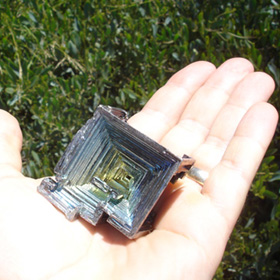 The image on the left is the third order variation of the Tetrabrot set. The photo on the right is a Bismuth crystal.
 |
4D Bicomplex Julia Set - C++, 7/29/09
 {x,y,z,w}2 = {x2-y2-z2+w2, 2(xy-zw), 2(xz-yw), 2(xw+yz)}
 |
Inverse 4D Bicomplex Julia Set - C++, 9/21/09


 These images were calculated using the inverse Julia set method. Dominic Rochon helped me with the formula for finding the square root of a bicomplex number. This formula has 4 roots, so the total number of points increases by a factor of 4 after each iteration. Here is some Mathematica code:
(* runtime: 0.7 second *) SqrtW[w1_, w2_] := 0.5{Re[w1] + Re[w2], Im[w1] + Im[w2], Im[w2] - Im[w1], Re[w1] - Re[w2]}; BicomplexSqrts[{a_, b_, c_, d_}] := Module[{z1 = a + I b, z2 = c + I d, w1, w2}, w1 = Sqrt[z1 - I z2]; w2 = Sqrt[z1 + I z2]; {SqrtW[w1, w2], SqrtW[w1, -w2],SqrtW[-w1, w2], SqrtW[-w1, -w2]}]; wc = {-0.2, 0.8, 0, 0}; wlist = {{1.0, 1.0, 1.0, 1.0}}; Do[wlist = Flatten[Map[BicomplexSqrts[# - wc] &, wlist], 1], {6}]; Show[Graphics3D[{PointSize[0.005], {Hue[#[[4]]], Point[Delete[#, 4]]} & /@ wlist}, Boxed -> False, Background -> RGBColor[0, 0, 0], ViewPoint -> {0, 10, 0}]] |
4D Julibrot Set - C++, 7/6/09
 The complex Julia set is typically calculated in 2D with a constant complex seed value. However, if you consider the set of all possible Julia sets (all possible seed values), you get the complete 4D Julibrot set. The Mandelbrot set is contained as a 2D slice of the 4D Julibrot set. You can also take 3D slices of the 4D Julibrot set as shown here. The left picture shows what the Mandelbrot set looks like if you vary the real part of the starting value along the third dimension and the right picture shows what it looks like when you vary the imaginary part. Technically, this is not a hypercomplex fractal, but it's still worth mentioning here. Here is some Mathematica code:
(* runtime: 18 seconds, increase n for higher resolution *) n = 100; Julibrot[z0_, zc_] := Module[{z = z0, i = 0}, While[i <12 && Abs[z] < 2, z = z^2 + zc; i++]; i]; image = Table[z = 1.5; While[z >= 0 && Julibrot[z, x + I y] < 12, z -= 3/n]; z, {y, -1.5, 1.5, 3/n}, {x, -2, 1, 3/n}]; ListDensityPlot[image, Mesh -> False, Frame -> False,PlotRange -> {0, 1.5}] |
 Links
LinksJulia Set in Four Dimensions - good explanation, by Eric Baird hypercomplex fractal gallery - by Jos Leys Julibrot discussion - on Fractal Forums cross-section showing Mandelbrot set - by Ramiro Perez Alien Interface - animated Julibrot with orbit trapping, by David Makin |
4D Hopfbrot Set - C++, 12/2/09
|

3D Exponential Mandelbrot Set - C++, 7/6/09

 This is what the Mandelbrot set looks like if you vary the exponent along the third dimension. It has a twisted shape because the features of the Mandelbrot set tend to rotate around the origin as the exponent is increased. Technically, this is not a hypercomplex fractal, but it's still worth mentioning here. Here is some Mathematica code:
(* runtime: 49 seconds, increase n for higher resolution *) n = 100; Mandelbrot[n_, zc_] := Module[{z = 0, i = 0}, While[i <12 && Abs[z] < 2, z = z^n + zc; i++]; i]; image = Table[y = 1.5; While[y >= 0 && Mandelbrot[z, x + I y] < 12, y -= 3/n]; y, {z, 1, 4, 3/n}, {x, -2, 1, 3/n}]; ListDensityPlot[image, Mesh -> False, Frame -> False, PlotRange -> {0, 1.5}] |
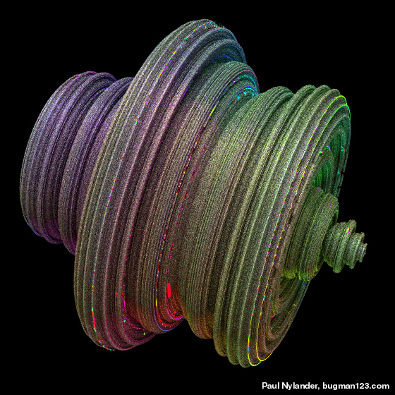
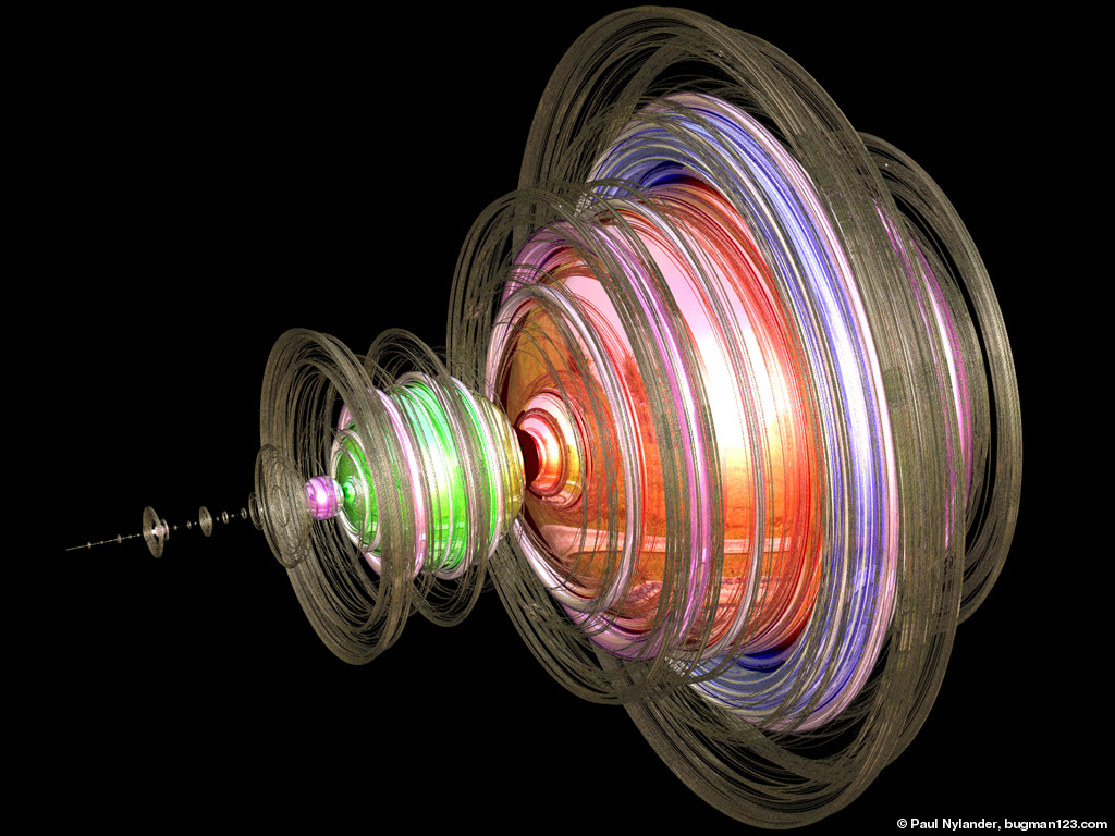
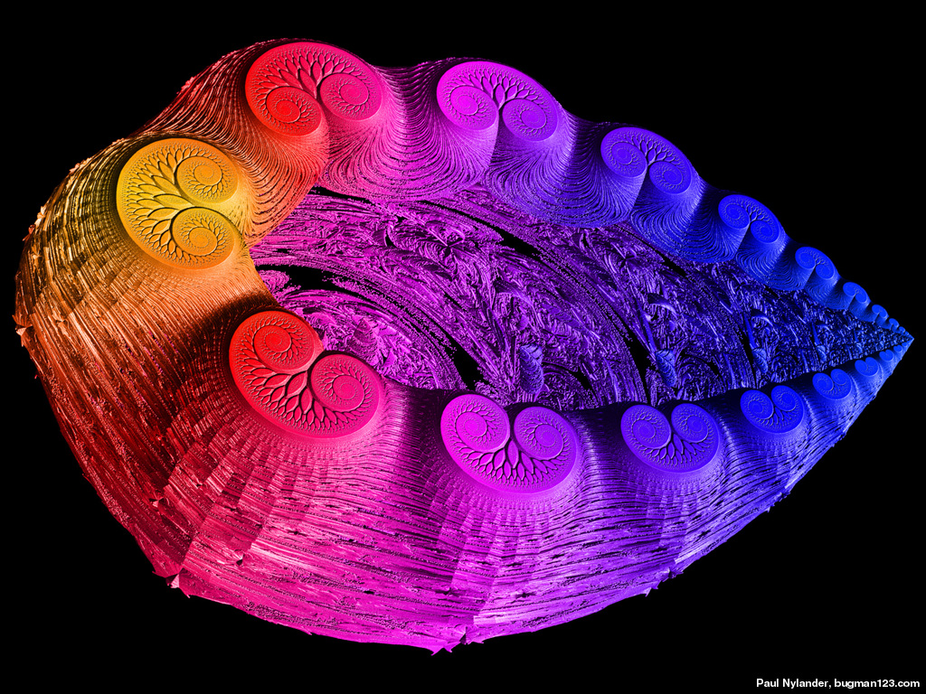
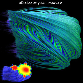
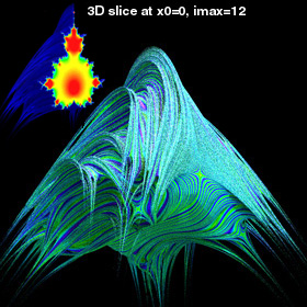
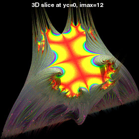
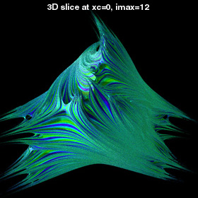
4D Mandelbulb Set - C++, 7/7/09

 Here is a 4D version of Daniel White's squarring formula. In 4D, rotation is about a plane and there are 6 possible rotational matrices to choose from: Rxy, Ryz, Rxz, Rxw, Ryw, Rzw. Following this train of thought, I came up with the following 4D analog to Daniel's formula by applying three consecutive 4D rotations:
{x,y,z,w}2 = Rxy(2θ)Rxz(2φ)Rxw(2ψ){r2,0,0,0}, r2=sqrt(x2+y2), r3=sqrt(x2+y2+z2), r=sqrt(x2+y2+z2+w2), θ=atan2(y,x), φ=atan2(z,r2), ψ=atan2(w,r3) This can be expanded to give: {x, y, z, w}2 = r2{cos(2ψ)cos(2φ)cos(2θ), cos(2ψ)cos(2φ)sin(2 θ), -cos(2ψ)sin(2φ), sin(2ψ)} This formula reduces to Daniel's squaring formula when w = 0 (which, in turn, reduces to the regular complex squaring formula when z = 0). For faster calculations, this formula can be simplified to: {x, y, z, w}2 = {(x2-y2)b, 2xyb, -2r2za, 2r3w}, a=1-w2/r32, b=a(1-z2/r22) Using this formula, I rendered 3D slices of this 4D Mandelbrot fractal at w = 0, z = 0, y = 0, x = 0. The animation shows the 3D slice starting from w = 0, and then rotating to z = 0, then to y = 0, then to x = 0, and finally back to w = 0 again. |
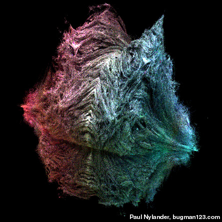
3D Nebulabrot - C++, 9/9/09

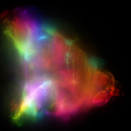
 The Nebulabrot is a variation of the Buddhabrot technique. These 3D variations were rendered from 2 billion points each. See also my 2D Nebulabrot.
Links Flying around 3D Nebulabrot - animation based on Daniel White's squarring formula, by Krzysztof Marczak |
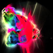
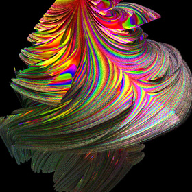
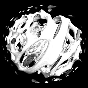
 Here are some volumetric renderings. This still has some bugs in it, but I think this will look quite beautiful if I ever get the bugs ironed out.
 |
3D Mandelbrot Set Orbit Traps - C++, 8/18/09


 Orbit trapping is a popular technique for mapping arbitrary shapes to 2D fractals. These images were created by extending this concept into 3 dimensions. These 3D orbit traps are shaped like spheres. See also my 3D Pickover stalks and 2D orbit trap fractals. Here is some Mathematica code:
(* runtime: 2 minutes, increase n for higher resolution *) n = 100; norm[x_] := x.x; TricornSquare[{x_, y_, z_}] := {x^2 - y^2 - z^2, 2x y, -2x z}; Clear[OrbitTrap]; OrbitTrap[p_] := 1.0 - norm[p]/0.3^2; Mandelbrot[c_] := Module[{p = {0, 0, 0}, i = 0}, While[i < 10 && norm[p] < 4 && (i < 2 || OrbitTrap[p] < 0.0), p =TricornSquare[p] + c; i++]; OrbitTrap[p]]; image2 = Table[z = 1.5; While[z > -1.5 && Mandelbrot[{x, y, z}] < 0.0, z -= 3/n]; z, {y, -1.5, 1.5, 3/n}, {x, -2.0, 1.0, 3/n}]; ListDensityPlot[image2, Mesh -> False, Frame -> False, PlotRange -> All] Links square orbit trap - uses formula for 8th order Mandelbrot set, by Enforcer 3D Mandelbrot set orbit trap - animation by David Makin Quaternion Eggs - I think this is a 3D orbit trap, by Ramiro Perez |
3D Mandelbrot Set, based on Rudy Rucker's formula for squaring a 3D hypercomplex number - C++, 9/6/09
 Rudy Rucker came up with this formula for squaring a 3D hypercomplex number in 1990. It is very similar to Daniel White's squarring formula, but differs in how one of the angles is calculated:
{x,y,z}n = rn{cos(θ)cos(φ), sin(θ)cos(φ), sin(φ)} r=sqrt(x2+y2+z2), θ=n atan2(y,x), φ=n atan2(z,x) The image on the right shows the 8th order variation of this fractal. Links Rucker Degree 2 - by David Makin |
3D Christmas Tree Mandelbrot Set - C++, 12/2/09
 {x,y,z}n = rn{cos(θ),sin(θ)cos(φ),sin(θ)sin(φ)}
r=sqrt(x2+y2+z2), θ=n cos-1(x/r), φ=n atan2(z,y) This 3D Mandelbrot set is based on a power formula that travels the same distance around the sphere no matter what the angle. The Cosine method also satisfies this requirement but one advantage of this method is that it reduces to complex arithmetic in the limit when z = 0 and therefore it contains the regular 2D complex Mandelbrot set as a cross-section in the x-y plane. This formula also happens to be identical to the 3D slice at y = 0 of my 4D Hopfbrot formula. |
3D Mandelbrot Set based on my attempt to combine the forward method with a reversed method - C++, 11/20/09

 {x,y,z}n = rn{cos(θ)cos(φ), sin(θ)cos(φ), cos(θ)sin(φ)}
r=sqrt(x2+y2+z2), θ=n atan2(y,x), φ=n sin-1(z/r) This was my attempt to combine the forward method with a reversed order method. The 8th order version looks like an explosion. |
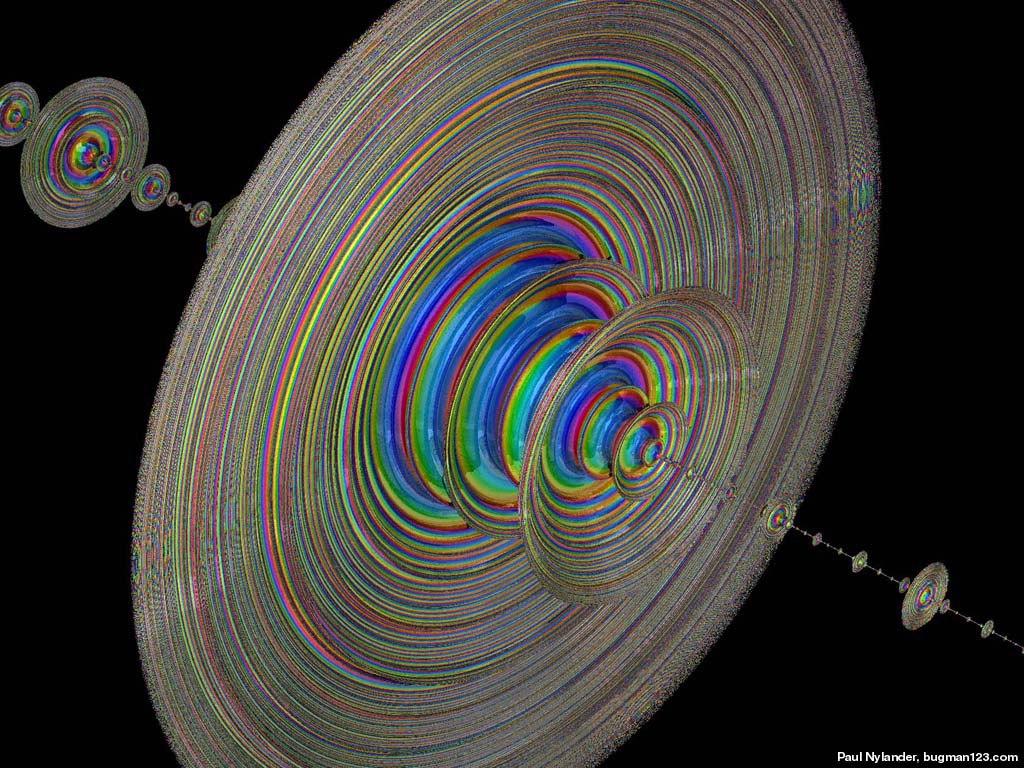
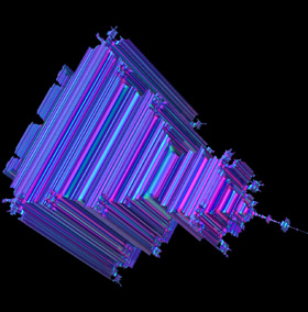
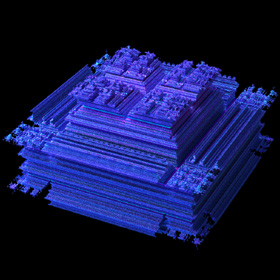
4D "Roundy" Mandelbrot Set - C++, 7/24/09
For a brief time, this formula was a popular method for creating 3D Mandelbrot sets. Here is some Mathematica code: (* runtime: 1.2 minutes, increase n for higher resolution *) n = 100; norm[x_] := x.x; RoundySquare[{x_, y_, z_, w_}] := {x^2 - y^2 - z^2 - w^2, 2 (x y + z w), 2 (x z + y w), 2 (x w + y z)}; Mandelbrot4D[c_] := Module[{q = {0, 0, 0, 0}, i = 0}, While[i < 24 && norm[q] < 4, q = RoundySquare[q] + c; i++]; i]; image = Table[z = 1.5; While[z >= 0 && Mandelbrot4D[{x, y, z, 0}] < 24, z -= 3/n]; If[z < 0, -1.5, z], {y, -1.5, 1.5, 3/n}, {x, -2.0, 1.0, 3/n}]; ListDensityPlot[image, Mesh -> False, Frame -> False, PlotRange -> {-0.1,1.5}] Links minibrot, Mandelbrot, Genuine Mandelbrot 3D, Minibrot 3D, New Mandelbrot 3D, True 3D Julia, Patch with Julia Fractals - volumetric renderings, by Krzysztof Marczak, be sure to see his animation Space Station - volumetric mini-minibrot, by Krzysztof Marczak 3D Mandlebrot - by Thomas Ludwig 4D Mandy, Minibrot - by David Makin |
4D "Roundy" Julia Set - C++, 7/28/09
 {x,y,z,w}2 = {x2-y2-z2-w2, 2(xy+zw), 2(xz+yw), 2(xw+yz)}
Links "Roundy" Julia Set - by David Makin |
Bristorbrot Set - C++, 12/4/09
 The Bristorbrot Set is based on the following formula for squaring a 3D hypercomplex number, as proposed by Doug Bristor:
{x,y,z}2 = {x2-y2-z2,y(2x-z),z(2x+y)} Links Fractal Dimension - Doug Bristor's blog Bristorbrot Set - discussion on Fractal Forums hypercomplex fractal gallery - by Jos Leys |
3D Mandelbrot Set, based on David Makin's formula for squaring a 3D hypercomplex number - C++, 10/14/09
 {x,y,z}2 = {x2-y2-z2, 2xy, 2(x-y)z}
David Makin suggested this formula for squaring a 3D hypercomplex number. It's kind of similar to the Bristorbrot. Links Mandelbrot Lightship - minibrot animation by David Makin |
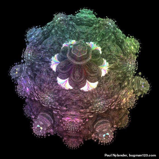
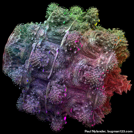
3D Mandelbulb / Juliabulb Sets, based on Roger Bagula's parameters - C++, 12/15/09
 Roger Bagula suggested these strange fractals to me based on Daniel White's squarring formula. I'm not sure if these would be considered Mandelbulb or Juliabulb sets.
 |
|
3D Mandelbrot Set - C++, 12/9/09


 The original Mandelbulb triplex power formula applies the azimuthal angle (φ) rotation away from the azimuthal axis (z-axis). However, one day I got confused and I thought that I had to sandwich the y-axis rotation between an un-rotate / re-rotate pair of transformations. Hence was born this formula.
Links Theme Park Ride - by David Makin |
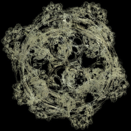
3D Mandelbulb Orbits - POV-Ray 3.1, 1/5/10
 Here is the boundary of the first orbit (3D cardioid) of the Mandelbulb, based on Daniel White's squarring formula. The image also shows the location of 3 roots for finding the second cycle 3D orbits, although I wasn't able to solve for the shape of those orbits. See also my 2D Mandelbrot orbits.
 |
4D "Squarry" Mandelbrot Set - C++, 7/30/09
 {x,y,z,w}2 = {x2-y2-z2-w2, 2(xy+zw), 2(xz+yw), 2(xw-yz)}
David Makin suggested this formula to me for squaring a 4D hypercomplex number. The right image is a zoom of the first miniature Mandelbrot set Links Mandy Squarry, Minibrot Squarry - by David Makin |
4D "Squarry" Julia Set - C++, 7/29/09
 {x,y,z,w}2 = {x2-y2-z2-w2, 2(xy+zw), 2(xz+yw), 2(xw-yz)}
c={-0.2,0.8,0,0}, imax=12 |
4D "Mandy Cousin" Mandelbrot Set - C++, 7/30/09
David Makin suggested this formula to me for squaring a 4D hypercomplex number. Links Which is Associated? - volumetric rendering, by Krzysztof Marczak Mandy Cousin - by David Makin |
4D "Mandy Cousin" Julia Set - C++, 7/29/09
 {x,y,z,w}2 = {x2-y2-z2+w2, 2(xy+zw), 2(xz+yw), 2(xw+yz)}
c={-0.2,0.8,0,0}, imax=12 |
4D Mandelbrot Set Variation - C++, 7/30/09
Here is another formula for squaring a 4D hypercomplex number that David Makin suggested to me. |
4D Julia Set Variation - C++, 7/29/09
 {x,y,z,w}2 = {x2-y2-z2-w2, 2(xy+zw), 2(xz-yw), 2(xw+yz)}
c={-0.2,0.8,0,0}, imax=12 |
Quadray Quaternion Julia Set - C++, 10/15/09
 Here is an unusal method that Ramiro Perez suggested to me. First it maps from a 3D point to a 4D quaternion by using negative and positive sides of tetrahedral space. Then it calculates the Julia set using quaternion math. Then it maps the final 4D quaternion back to a 3D point using quadrays. Finally, it applies an isosurface function to the resulting 3D point.
Links 3D Affine Transformation on 2D Inverse Julia - another cool way to create a 3D Julia set, by Ramiro Perez 3D Julia 1, 3D Julia 2 - by Ramiro Perez Quadray Papers - by Kirby Urner Quadray Formulas - by Tom Ace |
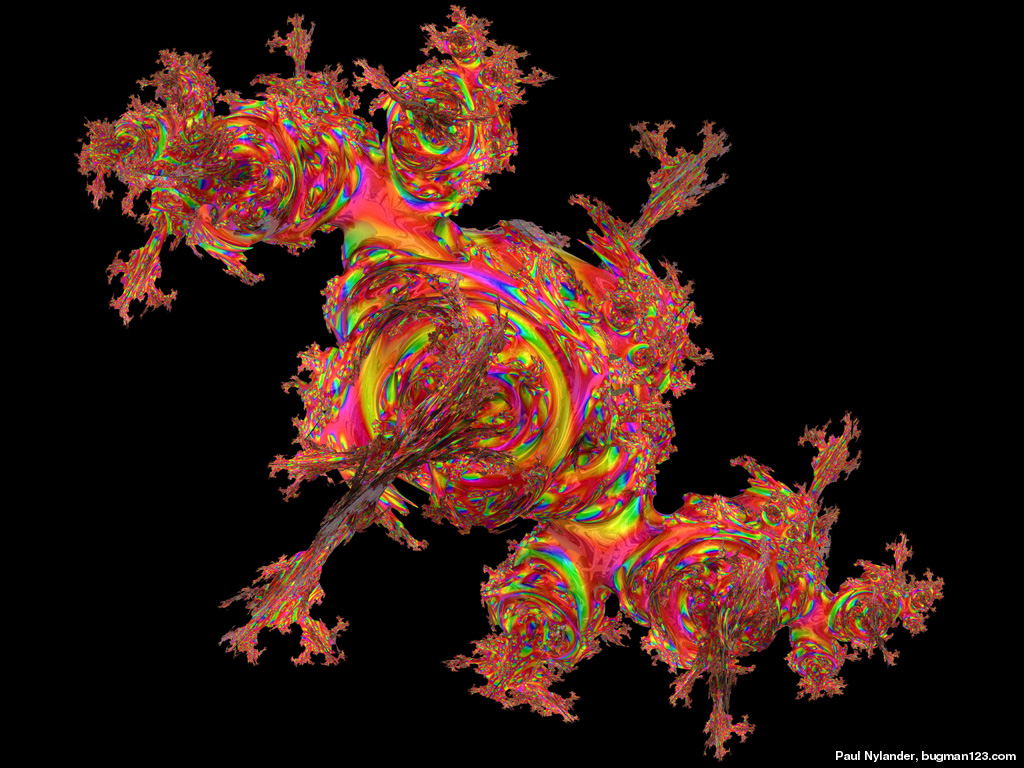
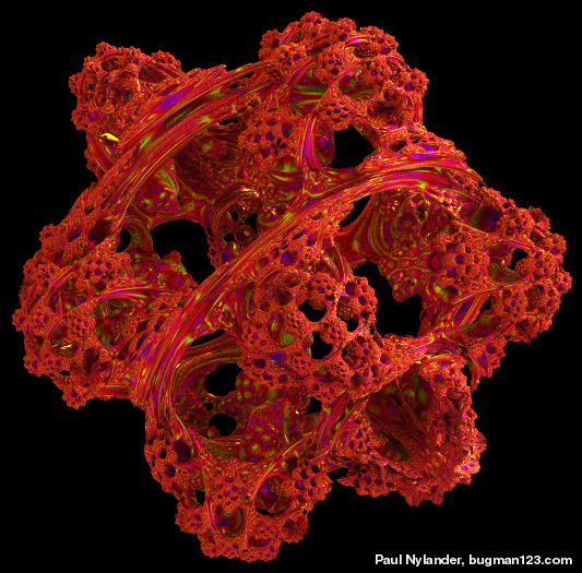
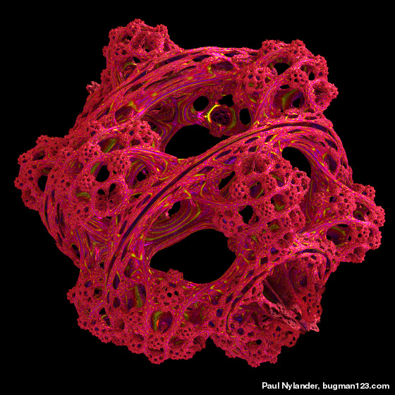
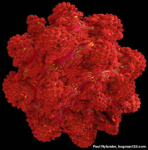
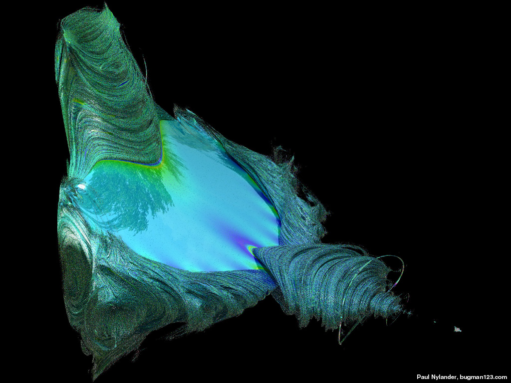
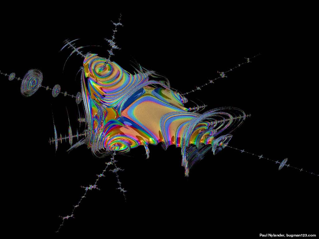
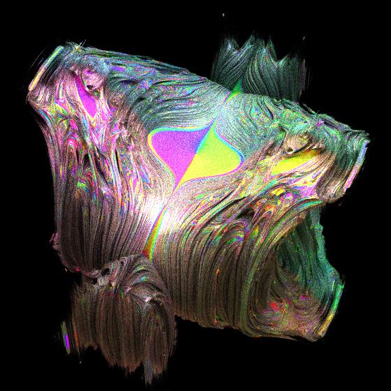
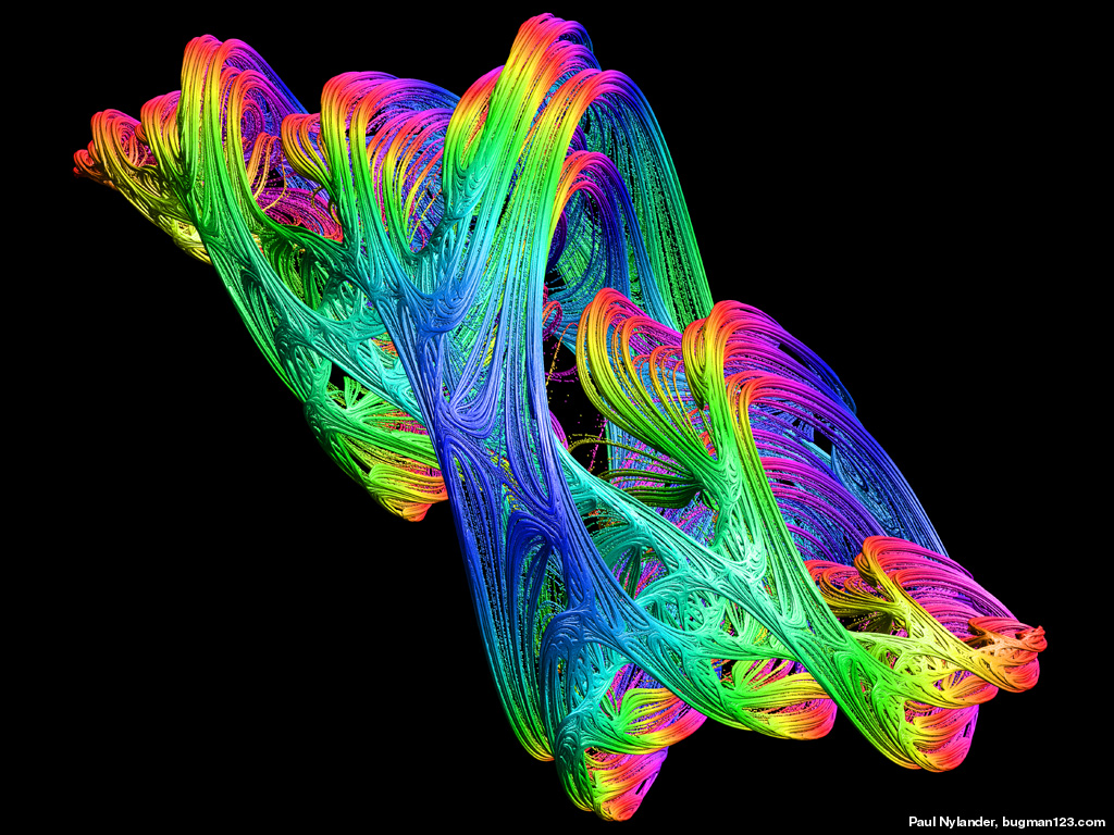
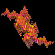
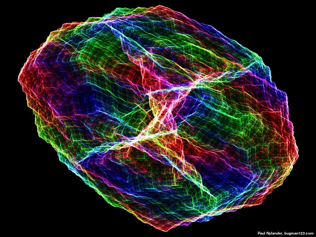
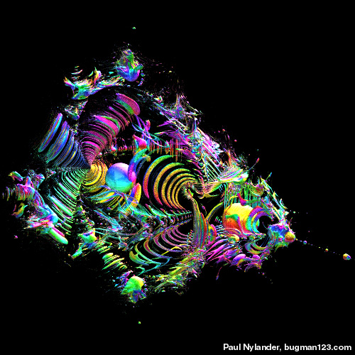
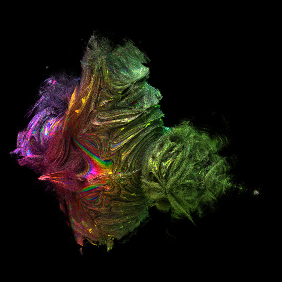
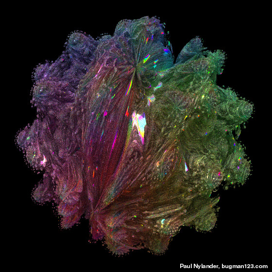
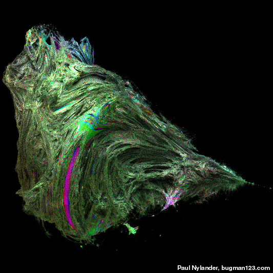
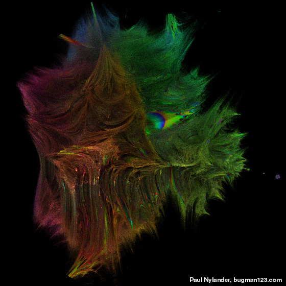
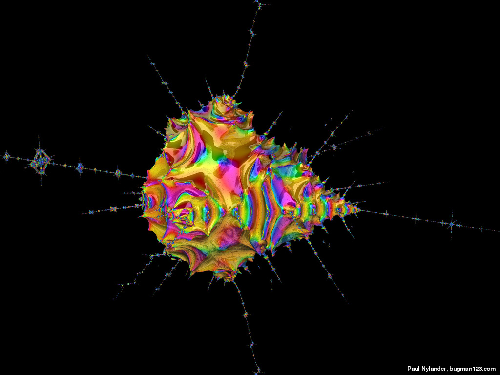
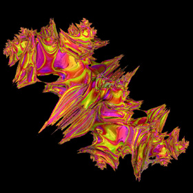
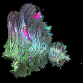
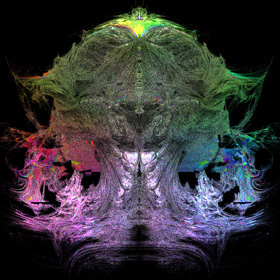
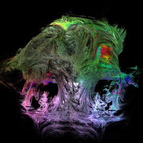
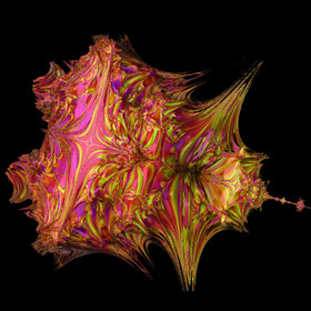
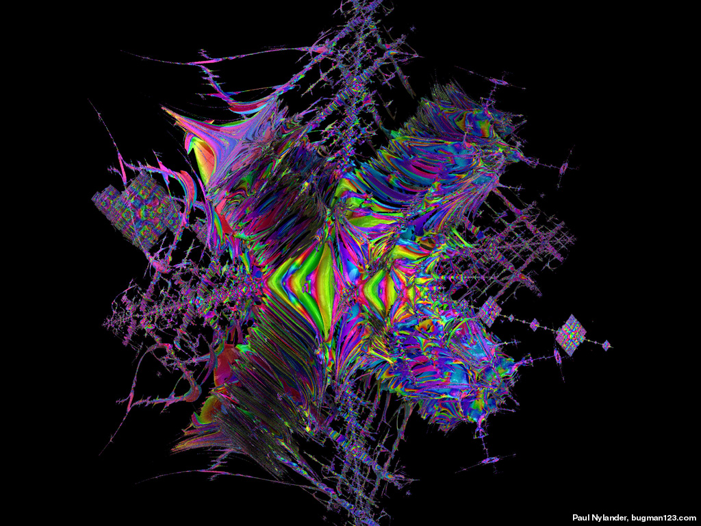
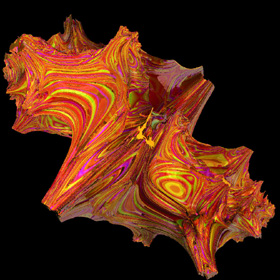
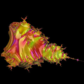
BoneYard - C++
 Here are some other weird looking hypercomplex fractals that I made while experimenting with different formulas. The possibilities are endless, but the challenge is to find formulas that produce intricate 3D details without looking like stretched out taffy.
|
Other Hypercomplex Fractal Links
3D Fractals - created by Richard Rosenman using Terry Gintz' QuaSZ software, includes "quaternion, hypercomplex, cubic Mandelbrot, complexified quaternion and octonion"